LiDAR to DEM Workflow

Using ArcGIS 10.0 to develop a LiDAR to Digital Elevation Model workflow for the U.S. Army Corps of Engineers, Sacramento District Regulatory Division
Author Zachary Fancher American River College, Geography 350: Data Acquisition in GIS; Fall 2012 email: zfancher@gmail.com Last Updated: 12/15/2012
Abstract It is the responsibility of the Regulatory Division of the U.S. Army Corps of Engineers to verify the jurisdictional status of aquatic resources, and to regulate permitting projects that impact jurisdictional waters of the U.S. Project managers are encouraged to make use of as many data sources as possible, but until recently, did not have access to high resolution LiDAR data for their areas of interest. After acquiring a 1-meter resolution LiDAR dataset encompassing a large portion of the Central Valley via a partner agency, the Sacramento Regulatory Division saw the need to develop a workflow that project managers could use to produce derivative Digital Elevation Models quickly when needed. This paper documents the pilot project used to demonstrate the value of LiDAR derived DEMs to the Regulatory Division, and the workflow needed to produce such surfaces. An analysis of the output files details ways in which the workflow can be streamlined, discusses accuracy and data verification, and offers alternate approaches to creating usable files. The paper concludes with a short discussion of the value of the derivative data, and directions its production may go in the future.
Introduction It is the responsibility of the Regulatory Division of the U.S. Army Corps of Engineers to conduct and verify wetlands/waters delineations, and to regulate the permitting process for projects that impact jurisdictional waters of the U.S. These tasks can involve the review and analysis of many different data sources; some in-house, and others generated by external agencies/consultants. The more accurate and complete the set of data for any particular site, the faster the Corps can make assessments, make decisions, and ultimately move forward with projects. Many times, the jurisdictional status of a particular feature(s) is not clear based solely on the documentation the applicant or consultant has supplied. Project managers often wish to use additional resources to clarify issues of land cover type, elevation change, hydrology and the like. At present, it is common for PMs to conduct field visits in order to gather the information they need to revise feature boundaries, add features that may have been missed, or subtract features entirely. However, over the last few years there has been increased encouragement from Regulatory Chiefs to do as much remote reconnaissance as possible, from the desktop. This is due to a number of reasons, including limited budget, limited staff and high workload. In order to make remote jurisdictional determinations a feasible option for anything other than the simplest of project sites, the need for remotely sensed data offering resolutions of an order of magnitude greater than that which has been used traditionally has become a necessity. Common data sources have included 7.5” USGS quad maps, USDA soil type maps, lower resolution aerial imagery, and of course consultants’ data sheets. Imagery available via Google Earth has increased tremendously in resolution over the last few years, and has been put to use frequently by the Corps. However, elevation data from GE is still not at a point where fine details can be discerned; hence it is not a reliable resource for accurately delineating aquatic features. With the increasing availability of remotely sensed LiDAR data, it has been suggested that Digital Elevation Models generated from LiDAR with sufficiently small point spacing could prove to be an invaluable tool for the Regulatory project manager. Recently, the Sacramento Regulatory division learned that the Engineering division had acquired a vast LiDAR dataset through a sharing agreement with the State of California Department of Water Resources. The LiDAR was generated as part of DWR’s Central Valley Floodplain Evaluation and Delineation Program, and was made available to Regulatory in the form of raw .las files. Many of the personnel in Regulatory are unfamiliar with ArcGIS 10.x, so it was determined that a pilot demonstration project coupled with a Standard Operating Procedure document would be the best way to introduce how to generate accurate DEMs from the raw files. This project documents production of these resources and offers suggestions on how production of derivative data could be streamlined in the future. It is important to note that new tools included as part of ArcGIS 10.1 make much of the following workflow obsolete. However, it will remain a viable workflow for Regulatory, as budget constraints have eliminated the option of upgrading to 10.1, at least for the foreseeable future. This paper also does not get into the option of processing all of the LiDAR and serving up the derivative rasters as a mosaicked dataset. We are looking into ways to host and access the entire dataset as rasters, but again, purchase of additional hardware or software tools is not an option for the Division at this time. For now, piecemeal production of DEMs for specific areas of interest was deemed to be the best approach when using this LiDAR dataset.
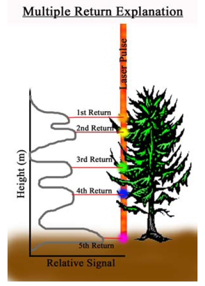
Background LiDAR stands for Light Detection And Ranging. It is a system that gathers remotely sensed data via analysis of the variable rates of return of laser light backscattered from an illuminated target. The primary components of a LiDAR system are: A) the laser, B) the scanner and optical system, C) the receiver and processing system, D) a geographic positioning system for georeferencing and correcting the collected data (Lillesand, Kiefer and Chipman 2008). A common method of obtaining LiDAR data is to fly an airplane carrying the above components over a target area while illuminating it with many thousands of laser pulses per second. Returning light will yield differentials from which elevations can be calculated. LiDAR systems commonly record multiple “returns”; that is to say, separate measurements for the light returning from discrete elevation layers (Figures 1a and 1b). These could be bare earth, canopy, understory, etc. The light will also return with various intensity levels. These return intensities can then be analyzed to yield information on material types.
Figure 1a	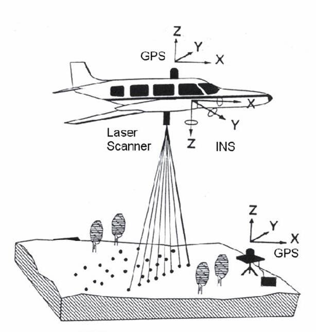Figure 1b
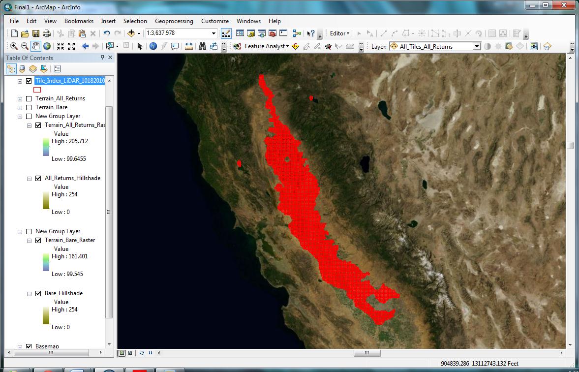
A wealth of electronic documents was supplied with the LiDAR dataset received by Regulatory. These documents provided most of the information on how the data was created, what equipment was used, what format and projection it was in, etc. Metadata files were also included, but I found that having the additional documents was critical for my understanding of the data. These included LAS Specification Version 1.1 (Igraham 2005), CVFED LiDAR_Orthos Comparison_052710 (Martinez 2011), Initial Post Processed LiDAR Product Sheet (Martinez 2012), and others. The primary sources consulted for information on raw LiDAR to Digital Elevation Model workflows were LIDAR_Processing_using_ArcGIS (Jennings 2009), and Lidar Analysis in ArcGIS 10 for Forestry Applications (Sumerling 2011). Both of these resources provided an overview of the basic steps needed to produce derivative data, and provided insight on how the process could best be tailored to fit the needs of the Corps. Remote Sensing and Image Interpretation (Lillesand, Kiefer and Chipman 2008) was also consulted for basic information on LiDAR data acquisition. The data was originally acquired in sections, from 2007 through 2010 (Martinez 2011), as part of a topography acquisition project headed by the California State Department of Water Resources. The intention was that the data, spanning a significant portion of the Central Valley (Figure 2), would be used to support hydraulic modeling and address flood risk as part of DWR’s larger Central Valley Floodplain Evaluation and Delineation Program (Martinez 2012).
Figure 2
The LiDAR data was broken up by DWR’s contractor into tiles, each measuring 5000’ by 5000’ (Martinez 2011). It was decided for purposes of the Corps pilot project that nine adjacent tiles would be used. This choice kept the processing time reasonable, yet still provided a wide variety of terrain to explore and analyze. The area of interest was chosen specifically for its relevance in the Sacramento District Regulatory Division; it is an area that historically has had a high density of vernal pool landscape, and has undergone much transformation over the years via agricultural conversion and development. The approximate center of the pilot project is at 38.864 N, -121.323 W (decimal degrees). The area of interest had to be chosen early on — as mentioned, different areas were flown at different times, and each area was given unique metadata. After settling on this location just southwest of Lincoln, California (Figure 3), I was able to consult its metadata for specifics on equipment, flight lines, and initial processing.
Figure 3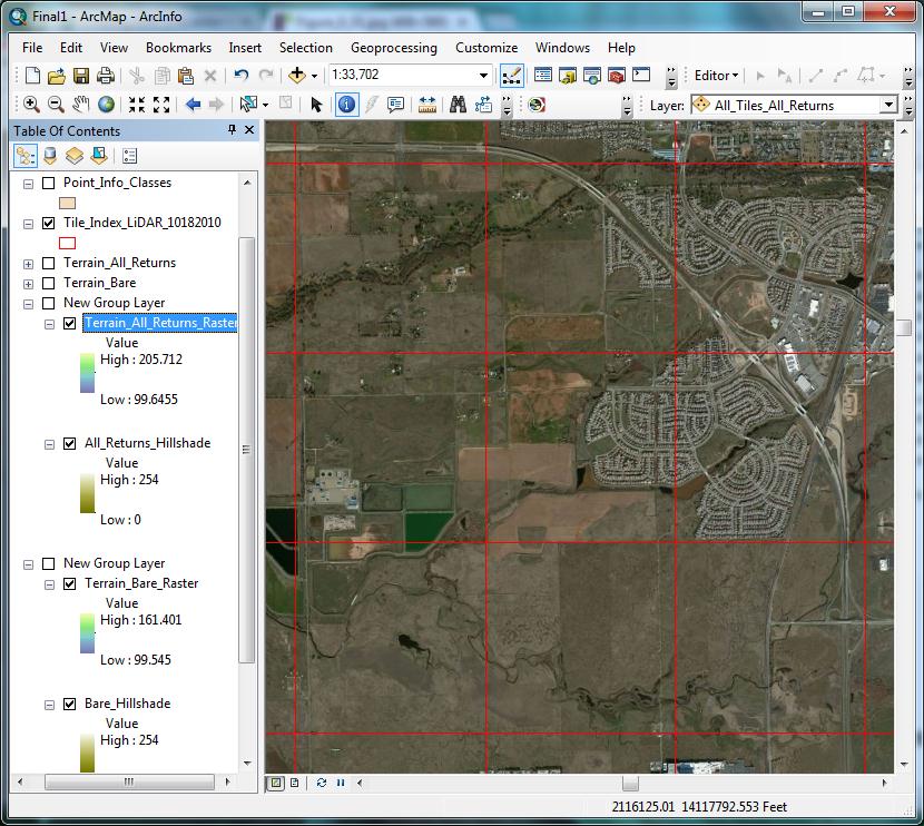
From the sources provided with the dataset and metadata specific to my project area, I was able to gather the following pertinent information: LiDAR Acquisition Contractor: Photo Science, Inc. Date Flown (for my project area): March/April 2008 Flight Line Overlap: 30% System Used: 2x Leica ALS50-II Datum: NAD 83 Projection: UTM Zone 10N, Unit = US Foot Vertical Datum: NADV 88 Accuracy: Accuracy - Vertical - 0.6’ Consolidated (1.96 x RMSEz), and 0.6’ Fundamental (95th percentile); Horizontal - 3.5’ (1.75 x RMSEx,y) Point Spacing (average for entire dataset): 3.28’ Coverage (for entire dataset): Approx. 9000 square miles Formats: LAS 1.1, ASCII (comma delimited) Data Verifications: -Data completeness and integrity -Data accuracy and errors -Anomaly checks through full-feature hillshades -Post automated classification -Bare-earth verification -RMSE inspection of final bare-earth model using kinematic GPS -Final quality control of deliverable products -Coverage check carried out to ensure no slivers present.
Methods Nine .las tiles were selected to represent an area of interest to the Corps, with a variety of water features, urban development, vernal pools and agriculture. Each tile measured 5000’ x 5000’, and the combined coverage represented an area of approximately 8 square miles. ArcMap was used as the production environment. The first step in the DEM production process was to create or choose a geodatabase to hold the data. A file geodatabase works fine for this purpose. The next step was to create a feature dataset inside the geodatabase. The feature dataset should be given the same horizontal and vertical coordinate systems as specified in the metadata or accompanying documentation. In this case, I used UTM Zone 10N (NAD 83) for the horizontal projected coordinate system, and NAVD 88 for the vertical. For ease of comparison against the documentation, I modified both systems to show linear units in Foot_US. The 3D Analyst extension is used heavily in this process, so it must be active. The tool 3D Analyst Tools > Conversion > From File > LAS to Multipoint was used next to convert the raw .las files into a multipoint feature class. The first DEM produced will be a bare earth interpretation of the point cloud. At this stage, all nine tiles were selected to participate. The average point spacing was set to 3.28, the average in feet for the entire dataset. The input class codes field was set to 2. This value was chosen using the LAS 1.1 specification for bare earth (Igraham 2005). The default of ANY_RETURNS was left checked in the returns field. The same coordinate systems used above were also entered. All other defaults were accepted (Figure 4). The resulting point cloud was (and must be) saved inside the feature dataset (Figure 5).
Figure 4
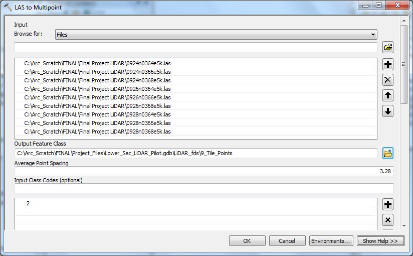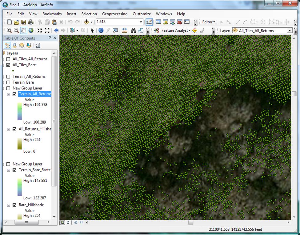
Figure 5 – Example (detail of resulting bare earth multipoint feature class)
The next step is to use the tool 3D Analyst Tools > Terrain Management > Create Terrain. The same average point spacing used above was inputted again, and the pyramid type was set to ZTOLERANCE as per recommendation (Sumerling, 2011). All other defaults were accepted. The terrain must also be saved inside the feature dataset. 3D Analyst Tools > Terrain Management > Add Terrain Pyramid Level must be used now in order for the terrain to draw properly. Values of 2 24000 were entered into the “Pyramid Levels Definition” field. The values represent window size and scale, respectively, separated by a space. All other defaults were accepted. Next, 3D Analyst Tools > Terrain Management > Add Feature Class to Terrain was used to get the terrain to reference the point cloud that was created earlier. Multiple feature classes can be added to and subtracted from the terrain as needed. In this case, only the bare earth feature class was used. The terrain was now built using 3D Analyst > Terrain Management > Build Terrain. NO_UPDATE_EXTENT was entered into the “Update Extent” field, because the terrain dataset is z-tolerance based (ArcMap Tool help file). Building the terrain now results in a surface that is very TIN-like in appearance (Figure 6). There are many geoprocessing options in ArcMap available to work directly from a built terrain.
Figure 6
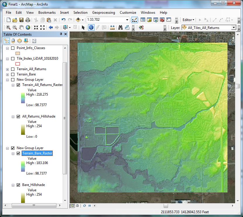
A DEM was created from the built terrain using 3D Analyst Tools > Conversion > From Terrain > Terrain to Raster. FLOAT was used as the output data type, to retain as much vertical precision as possible. NATURAL_NEIGHBORS was chosen for “Method”, as suggested in Lidar Analysis in ArcGIS 10 for Forestry Applications (Sumerling 2011). Sumerling wrote that this option produces smoother results overall, and while not as fast as linear interpolation, is more accurate. The “Sampling Distance” field is very important; this will receive more attention in the Analysis section, later. The default of OBSERVATIONS 250 was changed to CELLSIZE 3. This forces the output raster to be created with the specified cell size. “Pyramid Level Resolution” was left at 0, to retain full resolution at all scales. The DEM should be saved in the geodatabase, but not within the feature dataset. The resulting raster was symbolized using a stretched classification scheme; the stretch method used was standard deviations, n=2. The symbology was chosen to offer plenty of differentiation across elevation changes, while not being too hard on the eyes (Figure 7). In the display properties, the transparency was set to 45% in preparation for overlay over a hillshade raster, to be created in the next step.
Figure 7
A hillshade raster was created using the DEM raster as an input. Defaults were taken, and the resulting raster was also stretched using standard deviations n=2. The hillshade was placed below the DEM, resulting in the finished visual layer set for bare earth. These two layers were grouped to make turning them on and off easier (Figure 8).
Figure 8
All of the above steps were replicated for production of a DEM representing all classes, i.e. bare earth plus additional features like buildings, vegetation and canopy. The one step where values are modified from those used in the bare earth raster is the LAS to Multipoint step. To generate a multipoint feature class that contains all of the LiDAR, no input class codes should be entered. ANY_RETURNS should be left checked as well. A hillshade raster was generated from the resulting DEM. The DEM and hillshade should be grouped as before, and ordered above the bare earth group in ArcMap’s table of contents. Next, I did some finessing of the symbology and stretch standard deviation values in all four layers, such that when the canopy/buildings layer is turned on and off, it appears that only the canopy, vegetation, and buildings are being turned on and off. An imagery basemap was added, and the .mxd file was saved to the geodatabase. A Standard Operating Procedure document was produced, containing all of the above steps along with screenshots for all of the tool windows and preferred variables. File path names specific to the Sacramento Regulatory Division were included as part of the SOP. A shapefile containing the locations of all of the available LiDAR tiles (as in Figure 1, above) has been saved to Regulatory’s local drive, and can be used by project managers to determine which tiles they need to use in their DEM production workflow.
Results The DEM production workflow described above results in an easily transferrable high precision file geodatabase containing several derivative files. For each of the two layers, there is a multipoint feature class and a built, pyramided terrain (inside of a feature dataset). Inside the geodatabase, but outside of the feature dataset, there is a DEM raster and a hillshade raster – again, each for both the bare earth and canopy/buildings layers. These rasters are saved in FDGBR format, not as a preference, but simply because saving them inside the geodatabase allows for ease of transfer. In the future, should we wish to use the ArcGIS Server Image extension to serve up a seamless version of the entire LiDAR dataset, the rasters should be saved outside a geodatabase as .tif files, to aid mosaicking (Sumerling 2011). The elevation rasters are in a 32-bit format, to capture the full range of elevation values. The hillshade rasters are 8-bit, as only 256 values are required to represent the surface. Both the elevation and hillshade rasters are from continuous data sources. An .mxd file representing all of the derivative data as layers is included in the geodatabase. A single raw .las has an approximate average file size of 210 megabytes. At the cell size (3) used in the Methods section above, the resulting elevation raster for a single tile is approximately 10 megabytes. The hillshade raster is about 3 mb. Doubling these values to represent the bare earth and canopy/buildings layers, the total size is about 26 mb of derivative raster data per LiDAR tile. This is about 10% of the original .las tile size. This reduction is especially significant when contemplating possible rasterization and hosting of the entire dataset. The raw LiDAR files total at least 3 terrabytes in size!
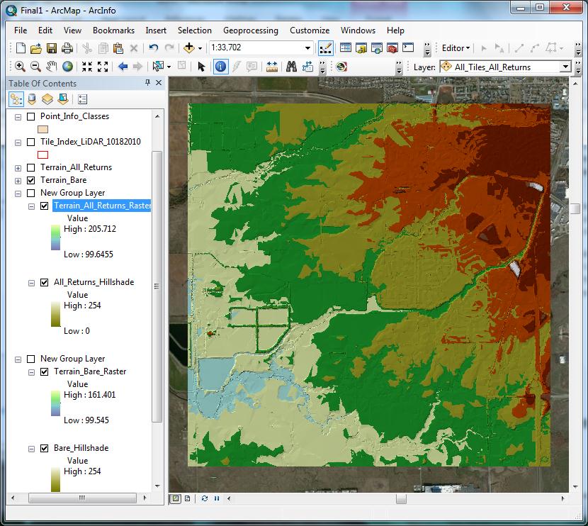
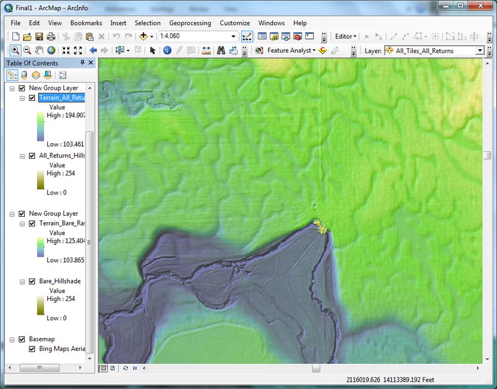
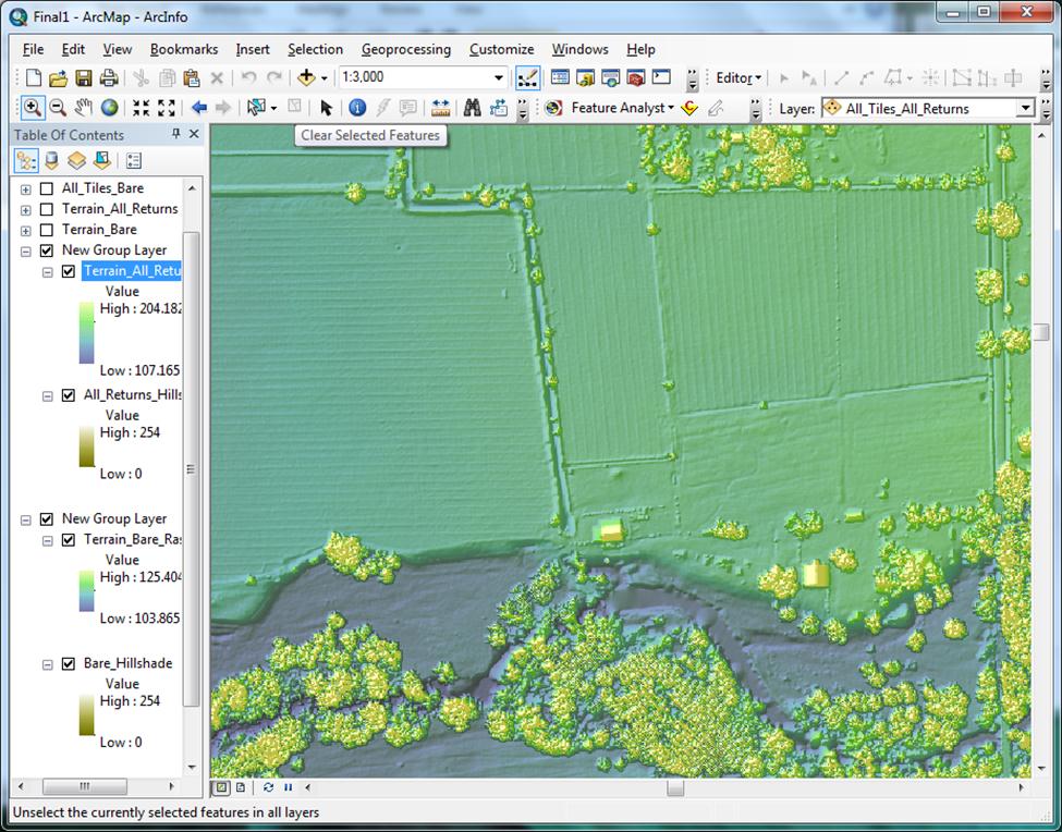
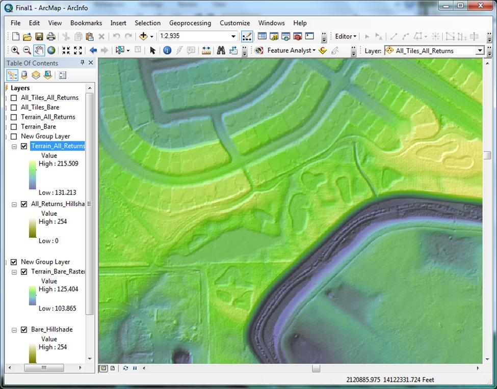
Analysis The derived surfaces are quite impressive, revealing watersheds, elevation changes, trails, terrain modifications, and other elements not discernible using other available data. 3 feet per cell is certainly seems to be a usable resolution for identification of most types of features of interest to a Regulatory project manager. I am confident these surfaces will become valuable resources in project managers’ arsenals (Figures 9, 10, 11).
Figure 9 - Example (canopy/buildings layer)
Figure 10 - Example (canopy/buildings layer)
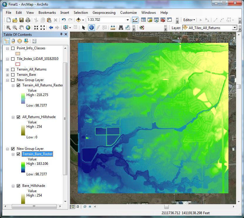
Figure 11 - Example (bare earth layer)
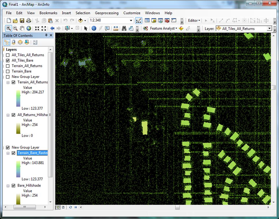
A visual quality check of the DEMs did reveal a few small areas exhibiting anomalies, though these were very infrequent and difficult to find. Initial data verification was conducted by Photo Science, Inc., with the goal of eliminating these anomalies, but apparently not all of them were caught. They appear as small “smeared” areas of non-existent topography, generally no more than 1000 square feet in size. I expected to see a degree of elevation difference between the bare earth DEM and the canopy/buildings DEM, owing to the interpolation taking place at the terrain to raster step. Using “Identify” on a selection of random pixels showed that the difference was actually very close – bare earth pixels on the canopy/buildings raster that were away from features that would affect the interpolation exhibited a range of about 0 to +0.1 foot difference from their bare earth raster counterparts. Pixels adjacent to vegetation and building features were on average about +0.12 of a foot higher than the same pixel on the bare earth raster. These differences are well within a workable range for the kinds of applications Regulatory will be using these rasters for. A cross check against Google Earth (which natively displays elevation only as whole numbers) showed the bare earth DEM to be accurate to within +/- 1 foot on average. The LiDAR elevation data was verified on delivery by Photo Science, Inc. to be accurate to within 0.6 of a foot at a 95% confidence level. My comparisons reassured me that only a small amount of acceptable error was introduced through production of the DEMs. Using the workflow described above produces detailed surfaces that convey quite a bit more elevation information than has traditionally been available to Regulatory project managers. That being said, there is an additional tool not described in the workflow, the use of which can help to provide even more detailed surfaces at higher resolutions. I found out about the Point File Information tool (located at 3D Analyst Tools > Conversion > From File > Point File Information) after I had already established the DEM production methodology, but have decided that use of this tool should now be the mandatory first step in the process. What this tool does is to create, for any .las loaded into it, a shapefile with an attribute table containing minimum/maximum z-values, point counts and average point spacing per .las file. Because every .las tile is unique, it has its own unique average point spacing – a spacing that is not represented when using the average spacing for the entire dataset (3.28 feet) at steps where point spacing is a required input. When testing many .las tiles in the middle portion of the Central Valley, I found the average point spacing of those tiles to be closer to ~ 1.8 feet. The pilot project tiles averaged around 1.7 feet. Running multiple tiles through the tool supplies the information needed to generate the average point spacing for just those tiles, and using that figure in the DEM production workflow would hypothetically result in a more accurate output. However, my testing revealed that changing the average point spacing value at the LAS to Multipoint step DOES NOT result in a multipoint file that is any different from the pilot project multipoint file. It is the exact same size, has the same number of points in the same locations, the elevations contained in those points are the same, etc. It is entirely possible that I am missing exactly in what way the average point spacing value affects the file and subsequent processing with that file, so I would still recommend using the best available value when prompted. The average point spacing given by the Point File Information tool does one other important thing though. It gives the analyst a value down to which they can comfortably reduce their raster cell size (Terrain to Raster step). Using this value for the cell size, the analyst can safely say that the cell size is representative of the average LiDAR point distribution, given an idealized single LiDAR point per cell. This also has the effect of giving the raster as much resolution as possible, with the minimum amount of data “made up” through elevation averaging. I have recommended in the SOP to take the value supplied by the Point File Information tool, round it to the nearest whole number (for the sake of ease in measurement and further analysis), and use it in the “Sampling Distance” field required in the Terrain to Raster step of the process. The reader may recall that the cell size of the pilot project output rasters was a value of 3 feet. 3 feet was chosen to satisfy the need for an integer (for ease of measurements and analysis), while still being as close to the 3.28 foot average point spacing as possible (for the best resolution). Remember that 3.28 feet is the average point spacing for the entire LiDAR dataset, and before I was aware of the Point File Info tool, it was the only value I could use to determine optimal raster cell size with any level of confidence. As mentioned earlier, use of this tool can reveal average spacing values that are different than 3.28, meaning a cell size of 3 is not necessarily optimal. The Point File Information tool can also differentiate individual classes, and give back statistics broken up by class. This is incredibly helpful. Before I learned of this tool, the only way to determine how the data was classified was through trial-and-error at the LAS to Multipoint step. In the case of this particular dataset, trial-and-error using class input codes specified in the LAS 1.1 specification were not producing any usable output aside from bare earth (class code 2) and all data (no class code). This was not an issue in the sense that these layers happened to be the ones I needed to meet project objectives, but for the sake of data comprehension, I wanted to know why entering class codes of 3 (Low Vegetation), or 6 (Buildings) was not working. To my surprise, running the Point File Information tool revealed that the data had only been classified as 1 (Unclassified), 2 (Bare Earth), and 12 (Overlap Points). Knowing how (and even if) the LiDAR data has been classified at the beginning of any DEM production can save time and frustration spent trying to pull out specific classes blindly. They may not even be present. When selecting returns (LAS to Multipoint step), only the value of ANY_RETURNS was chosen for both the bare earth and canopy/buildings rasters. This is the suggested method for modeling bare earth, and was also used for canopy/buildings, because bare earth was to be included in this raster as well. It was assumed that ANY_RETURNS coupled with no class code would generate a surface depicting everything illuminated by the LiDAR system, which did seem to be the case. In a potential use case where raw LiDAR data is classified better than the 1, 2 and 12 available to me, a different approach to generating the final data set would be in order. For the bare earth layer, LAS to Multipoint (class code 2, ANY_RETURNS) then Terrain to Raster (just like I’ve already done) would be appropriate. But for the canopy/building layer, LAS to Multipoint (class codes 3, 4, 5, 6, returns = 1) then Points to Raster (IDW) seems like a better approach. Class codes 3, 4, and 5 would bring back high, medium and low vegetation respectively, class code 6 would bring back buildings, and using the first return would ensure the maximum elevation of these features. Using Points to Raster (IDW) would create a canopy/buildings layer that could be symbolized to display ONLY the canopy and buildings, negating the need for the entire bare earth surface. So why is it that I was concerned with creating a canopy/vegetation layer at all, if Corps Regulatory’s primary concern is delineating water features? The answer lies in a visual exploration of the DEMs and multipoint feature classes. A glance at the bare earth multipoint reveals conspicuous areas where no LiDAR points are present (Figure 12).
Figure 12
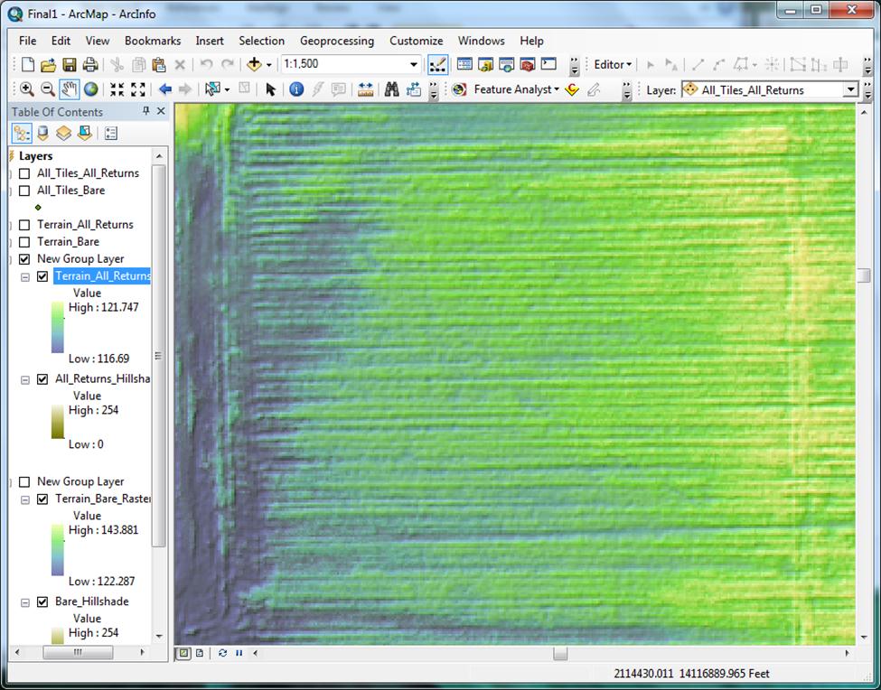
For the most part, these areas are water, man-made structures, and some areas of vegetation. When a DEM is produced from this point cloud, the point-less areas are interpolated from other nearby points, but the resulting surfaces in these areas do not model reality. They are areas of “no confidence” because in reality, those areas of bare earth are being obscured by vegetation and structures (Figure 13 – Bare earth exhibiting areas of “no confidence”).
Figure 13
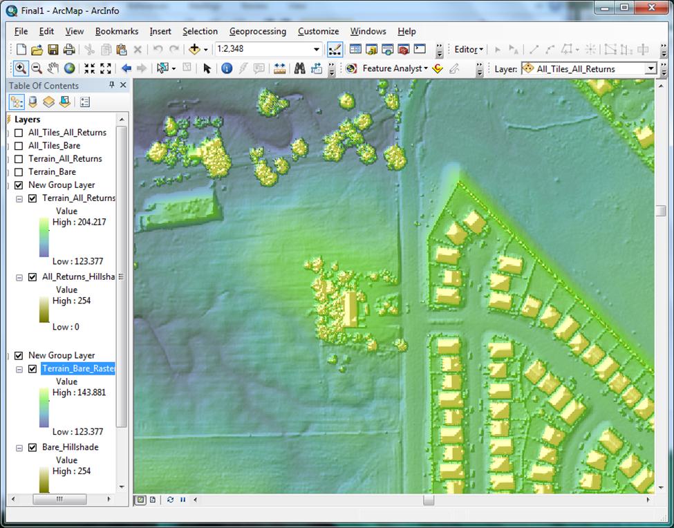
Because these areas are sometimes difficult to discern from the DEM raster, the need for another DEM that could show where they are became obvious. A project manager primarily needs to be examining the bare earth surface, but they also need to see where canopy and structures are, in order to quality-check their surface interpretations (Figure 14).
Figure 14
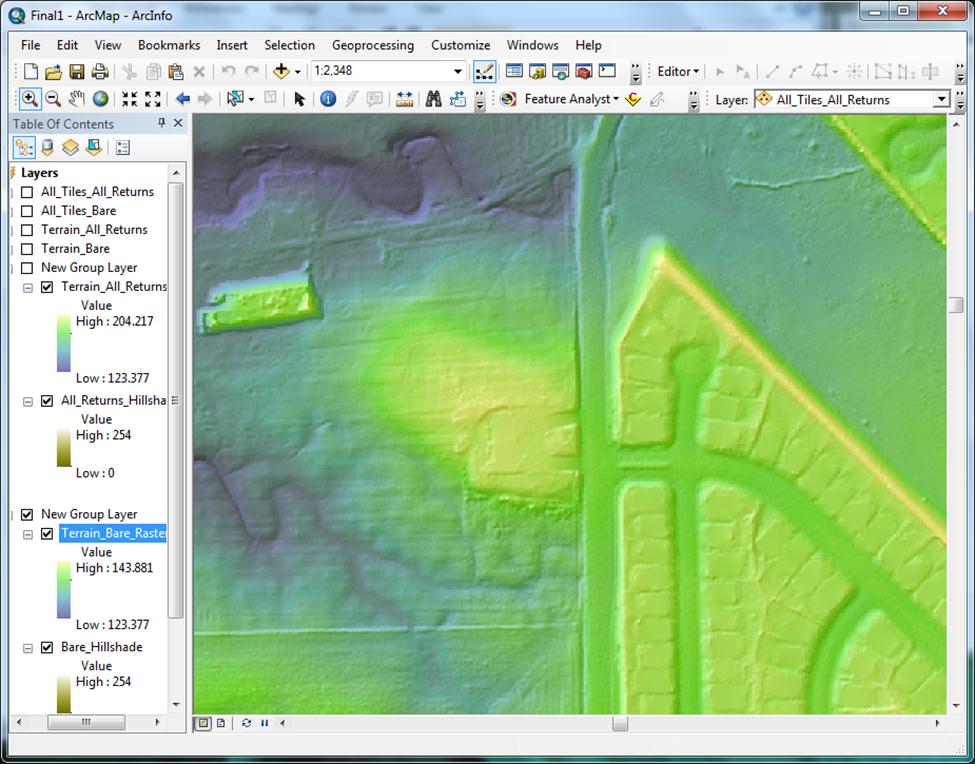
Sumerling suggests that the output raster cell size be set to four times the average point spacing of the LiDAR data (Sumerling 2011). I have seen this recommendation repeated in other LiDAR to DEM production workflows on the Internet. Jennings suggested that the cell size be set to 1/5 of the average point spacing (Jennings 2009). I believe this advice is for workflows that create elevation rasters via a direct point to raster operation. When using Terrain to Raster, I haven’t yet seen a good reason why the raster cell size should not be set to the same value as the average point spacing, aside from file size considerations or computing overhead incurred during analysis of high resolution raster DEMs. I will discuss the functional difference between these two methods further, below. I feel that Corps Regulatory, who will be analyzing only relatively small coverages, and who would gain a benefit from as much DEM resolution as possible, would be best served by setting the cell size value to that of the average point spacing of the coverage in question. This is of course, granting DEMs are being produced on a project-by-project basis. If multiple rasters were to be mosaicked later, they of course need to be set to the same cell size (the average spacing for all rasters in question). As I mentioned earlier, a DEM can be generated without the use of a terrain, via a direct multipoint feature class to raster surface operation such as IDW or Kriging. ESRI suggests that using a terrain provides more flexibility to add and remove features, and is more accurate overall. This is the reason that the terrain to raster method was chosen for this workflow. The Points to Raster operation produces a surface that, in the case of the bare earth class, contains many obscured areas that hold no data (places where there was overlying buildings or vegetation). The result is that the surface is full of holes with NULL values. This is visually distracting and not optimal for analysis. The cell size value of 4 times the average point spacing was suggested by Sumerling as a way to reduce NULL value cells and allow pixel averaging, though further processing is required to completely remove NULL values (Sumerling 2011). Given this information, the Terrain to Raster operation still seems most appropriate to apply to the Regulatory DEM production workflow. There is another important layer preparation step that I should mention. Before delivery to the project manager, both DEMs should be set to generate statistics from the current display extent (Layer Properties > Symbology > Statistics). This has the effect of applying the entire symbology color range to the extent of the view. The reason this is important is that it provides much more contrast in areas of little elevation change, so even in apparently flat areas, the PM can determine in what direction water will be moving (Figure 15).
Figure 15
A secondary effect is that the layer(s) in the Table of Contents will now update to show the range of elevation contained only in the display extent. An important caveat here is that depending on the scale of the image in the display, certain pixels can be obscured and will not be represented in the Table of Contents. Particularly at small scales, small areas of quick elevation change (a tall tree, for example) may not be represented in the TOC. Therefore, making elevation generalizations while using the TOC set to generate statistics from the current display extent should be done with caution. The best approach when needing specific elevation values is to turn this feature off, or better yet, use the “Identify” tool.
Conclusion Given that the U.S. Army Corps of Engineers Sacramento District Regulatory Division will not be upgrading to ArcGIS 10.1, the DEM production workflow outlined above is an excellent solution to the problem of how to utilize the raw LiDAR data. Analysis has shown both the primary and derivative data to be of high quality, exhibiting excellent accuracy at both the horizontal and vertical scale. Workflow improvements were identified, particularly mandatory use of the Point File Information tool to generate an average point spacing specific to the tile(s) being studied. We learned that raster resolution can be improved without additional loss of information, by using this same value when choosing raster cell size. Shortcomings in the dataset’s level of classification were identified, and an alternate method of producing a canopy/buildings layer from LiDAR that is fully classified was described. The use of return values with well classified data was illuminated. Finally a Standard Operating Procedure document was produced and stored on a drive at Sacramento District headquarters. Looking to the future, there a couple avenues to explore that may make production and delivery of these LiDAR surfaces quicker and easier. As mentioned, it is not likely that the ArcGIS Server Image extension will be purchased by our division anytime soon. It is for this reason that a project-by-project approach to DEM production is likely to continue for the foreseeable future. Given this reality, the next logical step would be to design a ModelBuilder tool or Python script to automate production of the derivative files. In fact, I built a tool using ModelBuilder for exactly this purpose. The tool was not a part of this paper however, due to the fact that I was only able to get it to work on a single machine. By definition, the tool needs to be a “shared tool” that can dynamically adapt to incorporate correct file paths for any computer it is used on. At present, my model has elements that use hard coded (not variable) file paths, so does not work as a shared tool. Python may be a better way to tackle automation of this task than Modelbuilder, but only further research will confirm this. At another end of the spectrum, Regulatory may be getting a full ESRI ArcGIS online license soon. We may be able to leverage this to host and serve the entire raster dataset, but again, this will take additional research.
References Igraham, 2005. LAS Specification Version 1.1. PDF white paper, 1:1-11. Jennings, N., 2009. LIDAR_Processing_using_ArcGIS. PDF white paper. American River College, 1:1-26. Lillesand, T. M., Kiefer, R. W. and Chipman, J. W., 2008. Remote Sensing and Image Interpretation. Sixth. (8.23):714-726. Martinez, J. C., 2011. CVFED LiDAR_Orthos Comparison_052710. PDF white paper. California Department of Water Resources, 1:1-2. Martinez, J. C., 2012. Initial Post Processed LiDAR Product Sheet. PDF white paper. California Department of Water Resources, Central Valley Floodplain Evaluation and Delineation Project, 1:1-1. Sumerling, G., 2011. Lidar Analysis in ArcGIS 10 for Forestry Applications. PDF white paper. ESRI Inc., 1:1-53.