| Title Ortho Mapping Workflow and Orthomosaic Creation | |
|
Author Levi S. Lebhart American River College, Geography 350: Data Acquisition in GIS; Fall 2018 w1388402@apps.losrios.edu | |
|
Abstract The project revolved around following the workflow as described in the Methods section of this document, borrowing from workflows for Historical imagery as derived by ESRI, in order to build a completed orthomosaic image that could then be used as a feature services within the ArcGis Online Environment. |
|
|
Introduction The goals of this project were to generate a basic workflow for orthomosaic creation using non-spatial data, resulting in a finished product to be used within the ArcGis Online environment. Other secondary objectives of this exercise were to become more proficient with the tools available within the ArcGis Pro platform as well as create better habits for data management. The main challenges faced during this project will be locating and downloading the necessary data, as well as metadata required for the generation of the orthomosaic. The process is also extremely time consuming- massive amounts of manual input to geo-reference the rasters, as well as applying proper pre-processing for the image files. Another issue comes down to the fact this imagery will most likely be non-spatial, requiring different procedures and protocols to be used within the ESRI suite of products. | |
|
Background Levi S. Lebhart is currently enrolled in American River College, majoring in Geographic Information Systems. He has currently completed the majority of courses within the program and is hoping to recieve his certificate in GIS after this fall semester. | |
|
Methods The primary workflow is as follows:
|
|
|
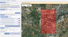
Data Collection USGS Earth Explorer The data was first collected from the USGS Earth Explorer, using a predefined shapefile in order to measure out the area of interest for the project. This geometry covered the majority of the Sacramento region, focusing primarily on the urban areas. The data that was collected were aerial single frames, at a scan resolution of 63 microns, 400dpi, with a scale of 1:15000. The photos were taken on May 9th, 2002, with a Carl Zeiss 153mm lens, and later scanned by the USGS and added to their archives in June 2017. The photo graphs were downloaded using the USGS bulk downloading applications they provide on the USGS website. The total disk space required by the files totaled 18 gigabytes, with 600 individual frames. |
|
|
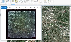
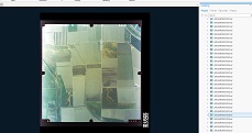
Pre-Processing Fix Orientation The downloaded imagery was improperly positioned for georeferencing, so it was re-oriented within Windows photo viewer. |
|
Pre-Processing Build Pyramids Once re-oriented, the imagery needs to have its raster pyramids rebuilt in order to reflect the changes within ArcGis Pro. |
|
|
Pre-Processing Define Projection The imagery had no spatial reference, so a batch process of "Define Projection" was completed in order to properly orient the imagery spatially within ArcGis Pro. This process was carried out with ArcCatalog. The fils were placed into a temporary file geodatabae titled "imageryRescale" in order to prevent them from becoming mixed in with the rest of the raw images. The files were then opened in ArcGis Pro. |
|
Pre-Processing Rescale ArcGis Pro has a simple tool that can be used for fix images whose extent do no fit with the current map the user may be currently working within, called "Rescale". The user interface within ArcGis Pro was far more intuitive for batch processing as well, allowing you to drop massive amounts of file into the data frame, and then start a batch process for multiple files with a simple click to add all of the files needed to be processed. |
|
|
Pre-Processing Clip Once rescaled, the images still had a black border from the previous scan of the photography that needed to be removed before further processing could be completed. A batch clip process was implemented to achieve this. The geometry for the polygon was derived by overlaying multiple items and finding out where they shared the most area. The final result was out put to a geodatabase called "ImageryCorrection", where much of the processing were to take place. |
|
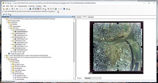
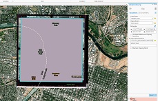
Georeferencing After pre-processing had completed the next portion was primarily used to georeference the entirety of the tiles. The tiles were georeferenced using a first-order polynomial transformation. These rasters were to cover the area as defined by the City of Sacramento "Neighborhoods" shapefile, as found on the City's Open Data Portal. The final count for rasters that had been georeferenced was 103 files, the rest of the files that had been processed as that point discarded and cleaned up. |
|
|
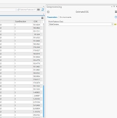
Compile Metadata Create Point Feature Class for Raster Centers The next portion of the project required collecting and creating the proper data needed to build the Frame and Camera tables for the mosacing portion of he process. The metadata that were collected were recommended by the ESRI workflow for historical imagery, which outlines a basic process for generating mosaic and orthomosaic imagery for imagery that is derived from older rasters. A new point feature class was created in order to accomplish this- the values that the point geometry would store would be used alongside the metadata to generate values for the photo laydowns "Course over Ground" (COG for short- the distrance that is travel by the plane with respect to a location on the ground). The metadata was compiled is as follows:
The definitions found above were derived from the ESRI Historical Imagery workflow, and the metadata collected from the USGS Earth Explorer, using the USGS data dictionary to interpret the values provided. |
|
Compile Metadata Derive COG Values The next step used the information derived from the metadata in order to provide the proper COG values to build the Frame and Camera tables for use with the Orthomosaic wizard. This was completed using the "Estimate COG Values" tool provided in the ESRI python tool box for the Historical Imagery toolbox. |
|
|
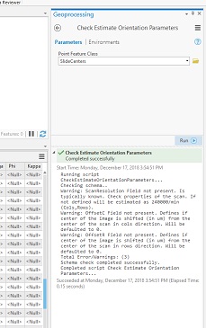
Compile Metadata Build Frame Table Once the COG value was derived, I could begin bulding the frame table. This was done by using the ESRI python tool "Check Estimate Orientation", as found in the Historical Imagery workflow. There were no errors, but two warnings while trying to attempt this, and the warnings were only to provide additional, optional data for the tool. I disregarded these warnings and went ahead with the process and used the next python tool titled "Estimat Orientation". The tool ran successfully, but only returned null values. |
|
Results
Orthomosaic
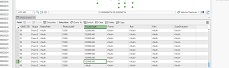
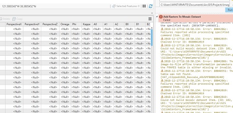
Even though the values provided were null, I still attempted to run the orthomosaic tool to see if it might generate something.
This resulted in nothing more than the fabled "Error 999999" reading. The tool was able to crawl and find the rasters however, only failing
when attempting to apply the table
| |
| |
|
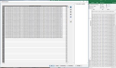
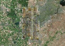
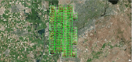
Mosaic Raster Footprints
Instead of an orthomosaic, I went ahead and build a mosaic raster foot print, which be used in various other processes to ortho correct
the imagery at hand. |
|
| |
|
Analysis The primary issue I believe occured while pre-processing the images. I ran comparisons on different
metadata finders for the images as raw files that had been downloaded from the USGS Earth Explorer, and then ran metadata finders for
the final images that were georeferenced and found a startling lack of information for the processed slides. Another issue I came up on were
gaps in the metadata from the USGS. I went all around looking for calibration reports for the cameras used only to find the page where
they store these to have last been updated in 2008. It was also an issue trying to track down who exactly took the photos, I searched USGS up and down,
the USDA, the National Archive and even Data.gov in order to find any inkling of idea of what project these images were from, but to no avail. The
agency that had been responsible for recording these images was only referred to as "Urban Area" which in multiple search engines from google, to duckduckgo, to bing
provided no specifics in regards to the USGS. The only item I was able to come across was a small tidbit from the National Map Small Scale. Using Archive.org provided
some insights here and there, but mostly just wound up being the same pages I had already seen, just with a different URL than the USGS uses now. |
|
|
Conclusions The files themselves would still be usable I believe. However they may need to be rescaled by means of the
scale tools found within the georeferencing tools in ArcGIS pro, and would have to raw, directly from the website as originally were, perhaps only defined for
a projection. I would have tried to contact someone in regards to interpretting the metadata provided by the USGS more clearly, and even possibly filed an FOIA
request for the calibration report for the camera that was used in capturing the aerial imagery, if it was neccesary. The general workflow regarding multiple geodatabases
worked well, however in reflection on the pre-processing methods it would be redundant, as much of those processes ended up harming the slides more than helping.
The final word
research. | |