1. INTRODUCTION

California has 100 million acres of land, farms and ranches occupy 30 million of them,   7.7 million acres produce crops.  Fresno County is the most productive agricultural county in the United States.   However in the last 20 years as population increased in the Central Valley, the agricultural land decreased, becoming urbanized. This report will be focusing on land use comparisons in Fresno County for the years 1986 and 1994. How many acres have been urbanized, what are some of the type of crops that have been lost due to urbanization, and why is this information useful and to whom?

The overall area of the study is the valley floor of Fresno County, bounded on the east by the Sierra Nevada foothills and on the west by the Coastal Range foothills. This report will cover 52% of the county as an overview and then focus on a quad size portion of the urban area of the city of Fresno.

2. BACKGROUND

When you hear statistics such as the state of California is expected to grow from its present level of 33 million people to 47.5 million people by the year 2020 you can imagine why it might be important to keep track of the land use. This population increase is expected to occur in the Central Valley where most of the food is grown and there is a large water demand. Water use is the purpose Department of Water Resources (DWR) conducts land use surveys.

In 1947, the State Legislature wanted an investigation of the water resources in California in an effort to predict the needs, present and future of the river basins. Compiling land use statistics is part of that process. Since 1950 the DWR has done periodic land use surveys of all 58 counties of California, focusing on irrigated agricultural land. DWR has completed 250 land use surveys in California as of 1997.

In the early years, surveys where done as needed, 1966 began a regular schedule of surveys that is presently in place although methods have changed due to the advances in technology. Land use surveys quantify the agricultural use by specific crops, crop groups, urban development, and native vegetation. The schedule rotates amongst the counties with emphasis placed on the counties that contain the most irrigated agricultural uses; these are surveyed every 5 to 7 years.

3. METHOD

In the earlier years of land use survey, the method used to calculate the acreage of agricultural land employed a method referred to as "cut-and weigh". This is a process of having a land use analyst go out in the field at the peak of the growing season and observe what crops are planted. Before the analyst did a site visit, aerial photos were taken and output to 35mm slides, which were projected onto quad sheets where field lines were delineated. The analyst would take the quad sheets in the field and identify the crop and make note of it on the quad sheet. This information was brought back to the office where the information was transferred to a second quad sheet. It was copied (the process of the day was referred to as sepia), and then the sepia copy was cut up along the field lines and then weighed, to calculate the acreage of the given crop. All the cut up pieces where placed in special envelopes that contained the weighed information and all the applicable land use and water source codes. These were then sent to data processing where all information was entered onto punch cards and a database was built.

The method employed in 1994 uses a method that more resembles GIS technology. GIS is rapidly changing, although for the 1994 land use survey the general process followed these steps:

a. Aerial imagery was obtained in the mid-growing season, typically late June or July. The imagery can be low (5500 ft) or high (18000 ft) elevation photography from an airplane, or satellite digital imagery.

b. Distinct fields, urban areas, native vegetation and major features were delineated from the imagery onto U.S.G.S. 7.5-minute quadrangle maps.

c. Land use codes were then assigned to the delineated areas, which were then verified through site surveys. Where multiple cropping was employed, more than one site visit was required.

d. Using AutoCad, the map lines were digitized and attributed.

e. Line work was checked, attributes were checked, and the data was aggregated into GIS format. Geographic Resources Analysis Support System (GRASS) software was used for the aggregation.

The projection used for the digitized maps is a customized Universal Transverse Mercator (UTM) that is referred to as CA105. UTM is used due to the property of the projection to maintain area. CA105 is a compromise between UTM10 and UTM11, this allows the entire state to be mapped in one zone. With software such as the DOS based Tralaine or a window’s software such as Blue Marble’s Geographic Translator, the CA105 projection can be transformed into other projections.

Aerial photos were taken from an airplane at an elevation of approximately 5500 feet and output into 35mm slides. The flight lines were one mile apart. In good weather it takes about 3 or 4 days of flying to cover 1million acres. This study area contains approximately 1.7 million acres.

The 35mm slides are organized into individual flight lines running south to north. Each slide is projected on a screen and field boundaries are manually delineated onto USGS quad sheets. For the Fresno County study area over 3500 exposures were required.

          Getting the line work digitized into the computer along with the attributes takes months to complete. As each quad is completed it goes through             a series of checks. The line work is checked for proper format for use in GRASS. The attributes are checked for proper format and accuracy.             The accuracy required is ± 60 feet at a 1:24000 scale. Taking into account that quads are ± 40 feet, the overall accuracy results in ± 100 feet.

IV. PROCESSING OF DATA FOR ARCVIEW USE

           After the quads have gone through quality control the data is:

• Exported from AutoCad as DXF files and attributes are ATT files
• Imported into Arc/Info and converted into coverages
• The coverages are exported out as e00 files
• The coverages are then made into shape files.

    The vector data is ArcView ready however the attribute files are not in the first normal form and require editing. In excel  bring in the attributes      as delimited text files. Having prior knowledge of the spread sheet data I was able to reformat the columns into first normal form so they would be      useable when doing queries.

V. THE RESULTS

    The following figure shows urban use comparisions:

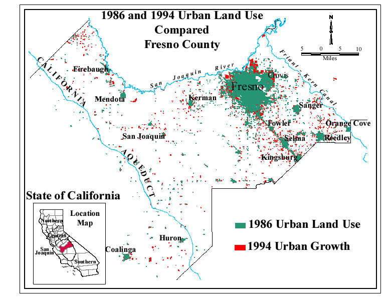alt="Urban Land Use in Fresno County 1986 Compared to Urban Land Use in 1994">

The following figure shows land use for the Clovis quadrangle:

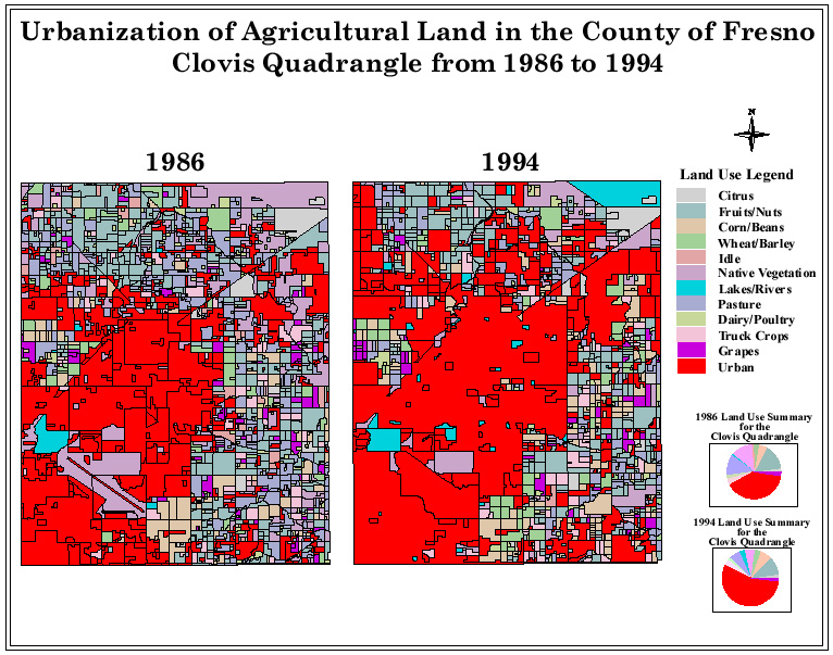
The previous figure shows the urban development for the Clovis area of Fresno.   From observation of the result, it appears that some of the areas previously classified as native vegetation in 1986, (particularly around the air strip) are classified as urban for the 1994 study.  Although this is not actually a loss of agricultural land it does illustrate that some classifications are subject to interpretation of the creator of the data.  This exposes some of the problems you can encounter when gathering datasets and the highlights the importance of metadata.

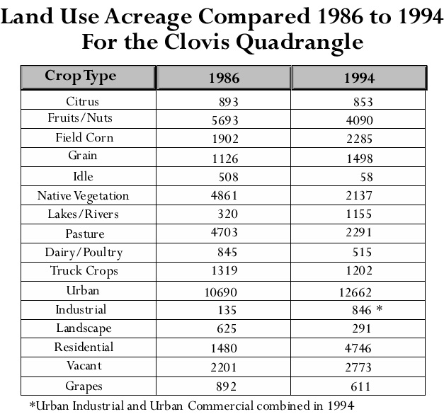
The figure below is a summary of the crop types from 1986 thru 1994 for the Clovis quadrangle:

The following graphic illustrates which land use types were urbanized:

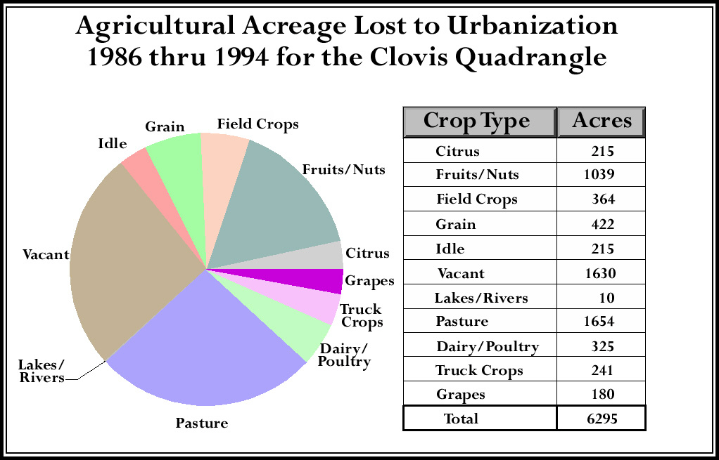
Based on this type of data that is collected, the state legislature is informed as to why water use is important to the Central Valley. The data is used, in part, to assist in verifying the water allocations, the prices, our water future, and the economy of the State of California.  Water affects so many aspects of our everyday lives.  It is liquid gold and the cause of many public debates.  Just try living without it.

VI.  REFERENCES:

San Joaquin District Staff and Division of Planning Staff 1994 Survey Report of Land Use in Fresno County, State of California Dept. of Water Resources, February 1997.

Dept. of Water Resources Land and Water Use Section Staff GIS and Data Format Standards for the Statewide Planning Program, State of California Dept. of Water Resources, December 1996.

Carter, Harold O. The Measure of California Agriculture, Its Impact on the State Economy, California Farm Bureau Federation, November 1992 (updated March 1996)

Pandol, J. and Chrisman, M. Report of the Agricultural Task Force for Resource Conservation and Economic Growth in the Central Valley, http://www.cfbf.com/agintro.html

Jones, J. "California Land Development Patterns", California Water Plan News March 1999.

Kasler, D. "Vanishing Farmland", Sacramento Bee, October 1998 http://www.sacbee.com/news/projects/farmlands/index.html

VII.  DATA SOURCE

Land Use Data: 1986 Fresno Land Use Survey and 1994 Land Use Survey, Department of Water Resources