Title

LOCATING OLIGOCENE-AGE ROCKS IN THE COAST RANGES: PATTERNS OF OCCURRENCE AND DISTRIBUTION

Author Information

Larry Hines

American River College, Geography 26: Data Acquisition in GIS; Spring 2002

Abstract

An attempt to conceive and plan a large geological study using GIS methods. Using GIS DATA FOR THE GEOLOGIC MAP OF CALIFORNIA, created generalized maps of outcrops of Oligocene-age rocks in California. Efforts to discern patterns of occurrence and distribution were unsuccessful. Methods and plans for further studies are discussed.

Introduction

Explore the use of GIS using geological problems, specifically, locating a defined category of rocks – Oligocene-age rocks within California, Analyze the outcrop pattern of the Oligocene rocks and consider what kinds of inferences may or may not be possible. This is a problem that I will only sketch using GIS methods; the "Oligocene problem " is a previous research interest.

Background

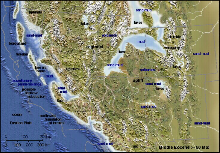
. The Oligocene Epoch (from 36 million years ago until 23 million years ago) is an interesting period in California’s geologic history for two reasons; a major shift in tectonics (plate motions resulting from the forces which drive Plate Tectonics), and the relative scarcity of Oligocene rocks (in California). The challenge of this problem lies in it’s scope and complexity: Oligocene sedimentary rocks which record characteristics of the paleoenvironment, contain fossils (ancient life forms), these, with other data, can be used to map a generalized paleogeography; and, more difficult, bring those rocks (the surviving record of ancient environments), through time and geologic events that may have altered, partially obliterated, or hidden them. To understand the project, modeling of Oligocene sedimentary environments, regional tectonics, local tectonic controls on sedimentary basin development, eustatic (sea-level) changes, paleoclimate models (climate affects erosion and sedimentary transport), and the direct rock and fossil evidence These are the main lines of evidence and reasoning, the hypothetical nature of much of the information makes it difficult to synthesize well-constrained models, however, different models could supported from the same general database. Realistically, with such a large and complex research topic, data collection would have to be disciplined; a few locations should be chosen (Oligocene outcrops) to study in detail. Also, analysis of a particular part of the Oligocene, possibly the close (end) of the epoch .is a more limited approach. The working hypothesis is that tectonics at the plate margin (San Andreas Fault zone) have hidden, translocated, largely obliterated, or restricted original deposition of the Oligocene rocks.

Methods

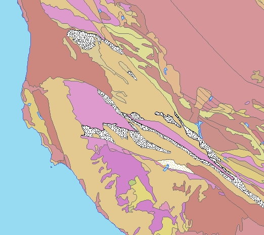
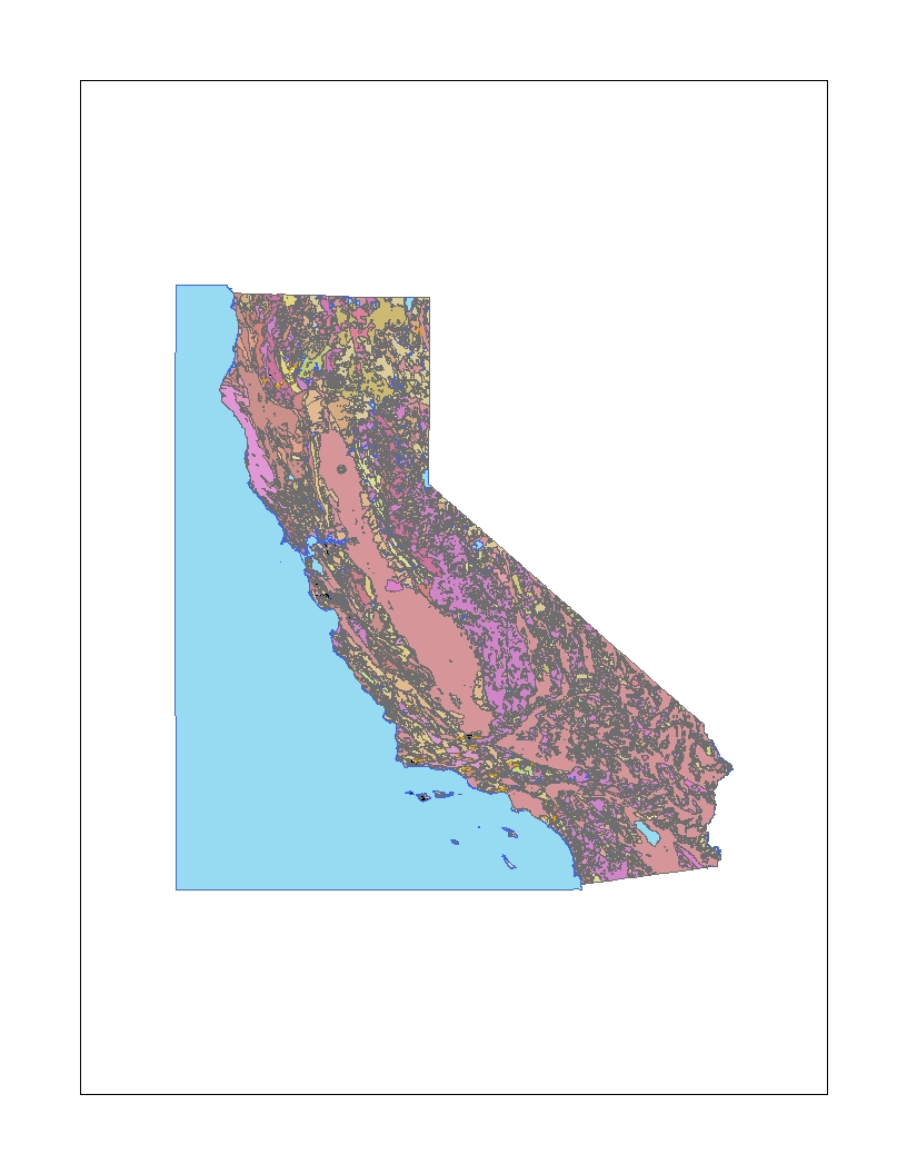
Available for this project is “GIS DATA FOR THE GEOLOGIC MAP OF CALIFORNIA, California Division of Mines,2000,CD. This contains digitized map,with a database of geologic units and faults that were created from tha Geologic Map of California,(Charles W. Jennings,1977). Already in ArcInfo export format this GIS was brought into ArcView 3.2. My original idea was to map the Oligocene rock outcrops and the rock strata above in time (Miocene rocks), and the strata below in time (Eocene rocks). Note the time span involved, the Eocene Epoch, 57 to 36 MYA, the Oligocene Epoch, 36 to 23 MYA, and the Miocene Epoch, 23 to 5 MYA. I concluded statewide project lacked validity, since there is great change in landforms geology, and tectonic regime across the different geomorphic provinces in California. The Coast Ranges of California is a very large area, and, the logical place to explore a genetic relationship between the San Andreas Fault zone and Oligocene rocks. Further, I would divide the Coast Ranges as follows: west of the San Andreas fault zone, east of the San Andreas fault zone, and the zone itself (in some areas) is a distinct entity; further subdivisions might have utility. Problems with the GIS map: the electronic format map is a digitized version of the 1977 Geologic Map Of California (scale 1:750,000), which is a generalized synthesis of Geologic Map Of California - a series of geologic maps done at a larger scale (1:250,000) and published between 1958 and 1969 (some of these maps were updated in the 1980’s). Since I was familiar with the older maps, I was confused until I purchased “AN EXPLANATORY TEXT TO ACCOMPANY THE 1:750,000 SCALE FAULT AND GEOLOGIC MAPS OF CALIFORNIA (Bulletin 201, CA Div. Of Mines and Geology, 1985), then I realized that the 1977 map took the 124 rock units of the older series and combined them into 52 units. This was disconcerting, because even on the 1:250,000 scale maps the rock units are generalized from more detailed mappings. A general technical confusion resulted from shifting back and forth between ArcView 3.2 and ArcGIS 8.1, neither of which I am proficient with. Figuring out the GIS map, bringing in the ArcInfo export files into ArcView and ArcGIS took time and help. I started to precisely color the map (the rock units on geological maps have unique colors based on conventions, American and International), something that can be done in ArcGIS, but won’t display in ArcView, so I discontinued. With more time, I would have cut a map of the Coast Ranges out of the map of California, and divided that map along the San Andreas fault zone

Results

Could not reach any real conclusions due to: generalized data; not enough subsurface data (rock units are 3-D); needed more information in general; and detailed information on the Oligocene rock formations. .

.

Analysis

After some consideration I saw the GIS map as a starting point, a tool for visualization and planning, the attribute tables supplied with the GIS map are very basic, but could be built up a great deal. While I could have done statistical comparisons [Oligocene as a percent of the Tertiary (by area or number of polygons), or compare Oligocene against Eocene], I felt this unreasonable, since my map showed outcrop area and number (polygons), if the estimated total volume rock was available for the respective Epochs, some tentative analysis could be started. In addition to the need to expand the GIS attribute table (database), I need to find a way to embed geological cross-sections on the map, ultimately, a 3-D map, and when available an animated model (to visualize fault kinematics and historical reconstructions of the Tertiary). The underlying difficulty was trying to choose a way to shape and present the project in such a way that it would make sense to the audience, the problem seemed too technical and esoteric (vague?), plus my approach of planning and conceptualizing a large, complex problem appeared to confuse people.

Conclusion

GIS concepts and thinking has shown a way to deal with complexity, has re-energized my thinking about a project I once considered overwhelming, and I see the inevitable and powerful impact GIS will have on geological studies - efficient geological reports and studies will assume a GIS format and be posted on the internet.

References

Ernst, W.G.,ed, 1981,Geotectonic development of California,: Rubey vol. 1

Ingersoll,R.V.,Ernst,W.G., 1987, Cenozoic basin development of coastal California,: Rubey vol. 6.

Jennings,C.W.,Burnett,J.L., 1961,Geologic map of California, San Francisco sheet,; CA Div. Of Mines and Geology, scale 1:250,000.

Jennings,C.W., ed, 1969 ,Geologic legend and formation indexes: part of series: Geologic map of California, CA Div. Of Mines and Geology, scale 1:250,000

Jennings, C.W., ed., 1977 Geologic map of California, CA Division of Mines and Geology, scale 1:750,000 .Jennings,C.W., 1985, An explanatory text to accompany the 1:750,000 scale fault and geologic maps of California,; CA Div. Of Mines and Geology, Bulletin 201

Saucedo,G.J., Bedford,D.R.,Raines,G.L., Miller.R.J., and Wentworth,C.M., 2000,GIS data for the geologic map of California, CA Div. Of Mines and Geology, CD.

Wagner,D.L., Bortugno,E.J.,1982,Geologic map of the Santa Rosa quadrangle, California: CA Div of Mines and Geology ;scale 1:250,000

Appendices

STANDARD GEOLOGIC TIME SCALE

EON	ERA	PERIOD	EPOCH	AGE (M.y.)	IMPORTANT EVENTS
PHANEROZOIC	CENOZOIC	Quaternary	Holocene	0.01 - present	Human civilization develops.
			Pleistocene	1.6 - 0.01	Continental glaciation in the northern hemisphere
		Tertiary	Pliocene	5.3 - 1.6	Humans appear for the first time.
			Miocene	23.7 - 5.3	Antarctic Ice Sheet develops.
			Oligocene	36.6 - 23.7	Himalaya Mountains begin to form.
			Eocene	57.8 - 36.6	The Alps form in Europe.
			Paleocene	66.4 - 57.8	Mammals become dominant land animals
	MESOZOIC	Cretaceous		144 - 66.4	Dinosaurs become extinct; Rocky Mountains begin forming.
		Jurassic		208 - 144	Atlantic Ocean begins to form between N. America & Africa.
		Triassic		245 - 208	1st dinosaurs; North America begins to separate from Africa.
	PALEOZOIC	Permian		286 - 245	All land masses joined to form a single supercontinent called Pangea.
		Pennsylvanian		320 - 286	Appalachian Mountains & Ouachita Mountains formed by continental collision with Africa.
		Mississippian		360 - 320	Extensive deposits of coal developed worldwide.
		Devonian		408-360	1st fossils of amphibians (animals which could live on land).
		Silurian		438 - 408	1st fossils of land plants.
		Ordovician		505 - 438	1st fossil fish; evidence of continental glaciation in Africa.
		Cambrian		545 - 505	Abundant fossils of marine organisms.
PROTEROZOIC	PRECAMBRIAN			2500 - 545	1st evidence of oxygen in atmosphere = 2.0 billion years ago.
ARCHEAN				4500 - 2500	Earliest evidence of life = 3.8 billion years ago. Earth forms = 4.5 billion years ago.