Title
GIS and Radar Rainfall Estimation
Author Information
Leiji Liu
American River College, Geography 26: Data Acquisition in GIS; Spring 2003
Abstract
Rainfall distributions from rain gages are typically estimated by assuming a
spatial geometry tied to point rain gage observations. Unfortunately, the
spatial distributions inferred by these approaches have little connection
with how rain actually falls. Since the release of the WSR-88D (NEXRAD) radar
in the early 1990s, many hydrologists and engineers have begun using gage-adjusted
radar rainfall estimates for hydrologic and water resource modeling.
Over large areas under multiple NEXRAD radar coverages, the quality of radar
rainfall estimates can vary significantly from one location to another. Visible
discontinuities can develop at the limits of coverage of a single NEXRAD
site because of slightly different performance or calibration techniques
used at the different radar sites. Using a variety of GIS procedures, these
discontinuities were eliminated and locations of ground clutter were suppressed,
yielding a seamless map of unadjusted radar rainfall estimates.
These data were adjusted with over 400 rain gages located throughout the state
of Florida. This approach was able to retain the volumetric rainfall estimates
from the gages while maintaining the spatial signature of the rainfall. Use
of this technique greatly improves gage-adjusted radar rainfall estimates.
Introduction
Radar has been used for rainfall estimation since 1940s, but only until 1990s,
after the WSR-88D (NEXRAD) system by National Weather Service (NWS) has been setup, did
serious application of radar rainfall estimation become possible. Radar
measures the electromagnetic power reflected by rain drops (called reflectivity).
The physical characteristics of radars and operational schemes create different
types of errors, and errors occur during the conversion from reflectivity to
rain rate as well. Scientifc research has found the relationship between
reflectivity and rain rate is not one-to-one relation, which means radar only
may not accurately estimate the rainfall, extra information is needed. Rain
gage data is usually used to serve this purpose.
Radar images give us a whole picture of the rainfall events and gage data
give us accurate rain amount at points. These points information is used to
adjust the radar images, resulting in better estimation.
Some problems related to the radar rainfall and gage adjustment are discontinuities
caused by the radar characteristics and operational options, significant topographic
constraint, and the mismatch of radar pixels and gages.
GIS system is used for visualizing the radar grid and images and checking errors.
Without GIS visualization pictures, some phenomena are hard to explain and understand.
Background
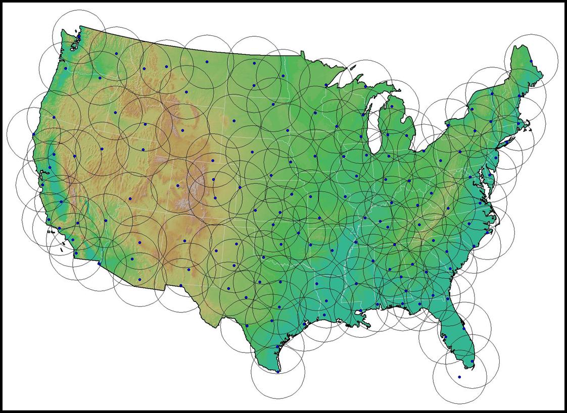
The NWS NEXRAD system consists of 142 radars covering the entire continental United States
(Figure 1). Each radar has about 230 km coverage. The whole image is a national mosaic of
individual radar coverages. NEXRAIN Corporation has the radar data with spatial resolution
of 2km by 2km and temporal resolution of 15 minutes from 1993 up to now, and radar data
with resolutions of 1km by 1km and 5 minutes interval from 2001 up to now. These data are
widely used in flood control, rainfall forecast, hydraulic and hydrologic designs, and
environmental monitoring, etc.
Figure 1: NEXRAD System
Methods
Since this project is not about the data processing and gage adjusted radar rainfall
algorithm study, I skip the details of the mathematics and physics applying on the radar
rainfall estimation and only present the problems and the possible solutions using GIS,
taking Florida as an example.
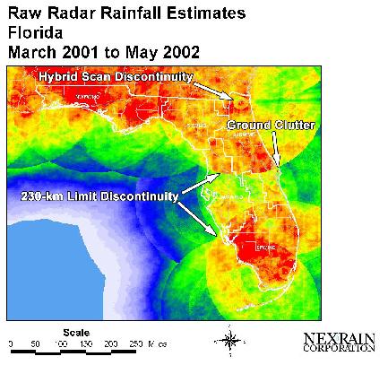
The first one is the discontinuities caused by radar scan (Figure 2). There are two
types of discontinuity. One is at the edge of the radar coverage, and the other one is
at about 10km distance, which is caused by so-called hybrid scan scheme. The data consists
of two or more scans. The base scan (elevation angle 0.5 degree) data is used only beyond
10km distance and within the 10km distance, higher eleveation angles data are used. This
scheme can solve some specific problem but it definitely creates the unnatural
discontinuity. In GIS, we record the pixel numbers of two sides of the discontinuity and
calculate an average ratio of the two sides and apply the ratio to one part of pixels.
The second problem is about ground clutter. When there are high buildings or mountains
on the path of radar scan, the reflectivity will be very strong, resulting in false
heavy rainfall (Figure 2). When we see such unusual high spots, we alway first load
the topographic maps into GIS and check if there is any mountain or building around the
study area. If we confirm there is, we use the average of surrounding pixels instead of
the false value.
Figure 2: 15-Month Radar Rainfall
Accumulation from March 2001 to May 2002
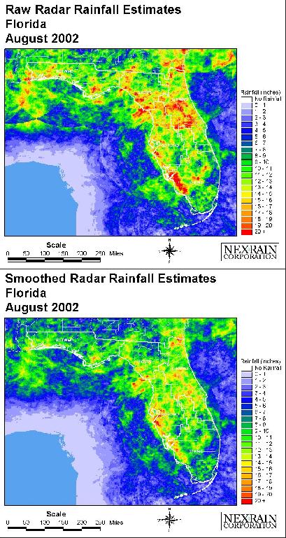
Figure 3 shows a comparison of images before and after smoothing.
Figure 3: Before (Raw) and After
(Smoothed) Radar Rainfall Estimates for August 2002
Results
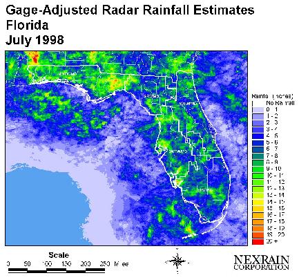
Figure 4 shows the gage-adjusted radar rainfall estimates for
the July 1998 study period. All discontinuities were removed
and the ground clutter was suppressed in the preprocessing of
the radar data by the GIS algorithms. The spatial adjustment
algorithm softly warped the radar rainfall estimates so that,
on average, the gage-adjusted radar rainfall estimates are very
similar to the rain gage estimates over each water management districts.
The algorithm also ensures that the spatial signature of the radar data is
not compromised.
Figure 4: Gage-Adjusted Radar
Rainfall Estimates for July 1998
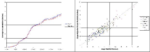
Figure 5 shows the average accumulation plot and scatterplot
for the 188 gages used in the analysis.
The average accumulation plot compares the accumulated average rainfall at
the rain gages (Gages) with the accumulated average gage-adjusted radar
rainfall at the radar pixels over the rain gages (Adj_Radar). The
Adj_Radar line closely follows the Gages line, indicating that, on average,
the gage-adjusted radar rainfall estimates nearly match the rain gage
estimates. The scatterplot compares the rainfall estimates at the gage
and at the radar pixel over the rain gage for each of the 188 gages
used in the study. The estimates do not line up on the 1:1 line, however,
there is a high degree of correlation between the two rainfall estimates
for all sets of data.
Figure 5: Average Accumulation (Left) and
Scatterplot (Right) Results for July 1998
Table 1 gives a summary of the average total rainfall at the gages
versus the average total gage-adjusted radar rainfall estimates at
the radar pixels over the rain gages for July 1998. In total, the
gage-adjusted radar rainfall estimates for July 1998 were about 3% less
than the rain gage estimates.
Table 1: Results (inches) for July 1998
|
|
Gage
|
Adj_Radar
|
Difference
|
|
NWDWMD
|
12.24
|
12.30
|
1%
|
|
SFWMD
|
6.06
|
5.67
|
-6%
|
|
SJRWMD
|
7.21
|
6.98
|
-3%
|
|
SWFMWD
|
8.03
|
7.76
|
-3%
|
|
NWS
|
7.29
|
7.14
|
-2%
|
Conclusion
1. The authors were able to remove discontinuities in the radar rainfall database
using GIS algorithms. These discontinuities are evident in the mosaiced dataset
that was used for this analysis, but the hybrid scan discontinuity will also
be visible will data from a single WSR-88D.
2. For any gage-adjusted radar rainfall analysis, review of the gage data
quality is extremely important.
3. For this study, the use of a large radius of influence with a spatially variable
adjustment algorithm is an appropriate method to create a gage-adjusted radar
rainfall dataset over a large area. Even though a large radius was used,
the gage-adjusted radar rainfall estimates at individual locations within the
]state matched very well with rain gage estimates.
References
Brandes, E.A. 1975. "Optimizing Rainfall Estimates with the Aid of Radar."
J. of Applied Meteorology, 14(7): 1339 - 1345.
Fulton, Richard A., Jay P. Briendenbach, Dong-Jun Seo, Dennis A. Miller, and
Timothy O'Bannon. 1998. "The WSR-88D Rainfall Algorithm." Weather and
Forecasting, 13: 377-395.
Hoblit, Brian C. and David C. Curtis. 2000. "Next Generation Rainfall Data."
Proceeding from the ASCE Watershed and Operations Management 2000 Conference,
Ft. Collins, CO.
Hoblit, Brian C. and David C. Curtis. 2001. "GIS Highlights Importance of
High-Resolution Radar Rainfall Data." Proceedings of the Twenty-First Annual
ESRI International User Conference, San Diego, California.
Hoblit, Brian C., Leiji Liu and David C. Curtis. 2002. "Extreme Rainfall
Estimation Using Radar for Tropical Storm Allison." Proceedings of the EWRI
2002 Conference on Water Resources Planning and Management, Roanoke, Virginia.