| Title The Socio-Economics of Crime: Burglary in Washington, D.C. | |||||||||||||||||||||||||||||||
|
Author Neil Dhawan American River College, Geography 350: Data Acquisition in GIS; Fall 2003 | |||||||||||||||||||||||||||||||
|
Abstract Identifying and quantifying spatial relationships between areas of high burglary density and various demographic characteristics. | |||||||||||||||||||||||||||||||
|
Introduction The root causes of crime have been well theorized and debated. An interesting corollary to this discussion is an examination of the relationship between geography and crime. Rather than attempt to identify what factors lead to crime, we may explore what factors accompany crime. That is, we focus on correlation rather than causation. This study attempts to do just that. In particular, I have attempted to quantify the relationships between various socio-economic conditions and areas with a high density of burglaries. Washington D.C. burglary data from the year 2000 was used in this analysis. By comparing the percentage of areas in close proximity to burglary locations that fall in census tracts with some measurable demographic value to the percentage of the city those tracts comprise, possible spatial relationships were identified. GIS’ ability to model such relationships, particularly in the raster file format, made it an excellent tool in this endeavor. | |||||||||||||||||||||||||||||||
|
Background Each year, the FBI publishes Crime in the United States, a statistical summary of crime offenses in the U.S. It merely provides a reference for crime statistics broken down by political jurisdiction and individual agency and, as such, the FBI warns that it should not be used as a singular tool of crime analysis. Different areas can have vastly different demographics; it is naďve and imprudent to think that crime rates do not need to be standardized in some way. However, the FBI does note that several crime factors are known to affect both the type and amount of crimes committed. These include but are not limited to:
| |||||||||||||||||||||||||||||||
|
Methods All spatial datasets were obtained from the ESRI website in the shapefile format. These included Washington D.C. census tracts, streets, major roads, water bodies, and 2,531 burglary locations for the year 2000. Because the census tracts shapefile was unprojected and did not have a projection file (*.prj) associated with it, I used ArcToolbox to set the spatial reference to the NAD83 Geographic Coordinate System. To eliminate any accuracy errors associated with data projected “on-the-fly” during an ArcMap session, I projected the census tracts shapefile to the NAD83 State Plane Maryland Projected Coordinate System to match the rest of the data. Since the area of each tract was not listed in the attribute table (an attribute I would need in my analysis), I created a Personal Geodatabase file (*.mdb) within ArcCatalog, and imported the census tracts shapefile in as a feature class to the Personal Geodatabase. This automatically created a field that contained the area of each census tract in square meters. Aerial photos were downloaded from the TerraServer USA website in a JPEG format. Although the photos were projected and came with GIS world coordinates embedded in a World file (*.jgw), I had to set the spatial reference to UTM Zone 18 (NAD83 datum) using ArcCatalog.Demographic data was downloaded from the U.S. Census Bureau’s American FactFinder website. The socio-economic information I obtained included the following:
This data was summarized by individual census tracts and downloaded as an MS Excel spreadsheet (*.xls). I imported this spreadsheet into MS Access as a database table, and created several new fields based on the existing demographic data and the census tract area field created in the Personal Geodatabase. These new fields included:
I exported the updated database table as a dBase IV (*.dbf) file, and added it to ArcMap. I then added all the D.C. spatial data, including a dBase IV table of pawnshop addresses in Washington, D.C. I geocoded the pawnshop locations and performed a tabular join between the demographic data table and the census tracts shapefile based on a census tract ID field. Because the
burglary shapefile contained point-specific burglary locations, there was a
possibility that relevant spatial relationships would be overlooked. That is,
if a burglary is committed near the border between two or more census tracts, I
needed a method to ensure that all census tracts in close proximity would be
included in the analysis of that particular crime event. This was done by
creating a straight-line distance GRID raster of 50 meters from each burglary
location.
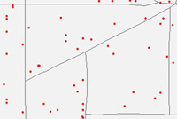
Burglaries as Points
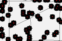
Burglaries as Burglary Proximity Zones In order to quantify (at least on some level) the relationships between burglary and certain demographic characteristics I utilized a simple process of topological overlay using the ArcGIS Spatial Analyst extension. Generally, the same basic steps were followed in each analysis: (1) Creation of a GRID raster file from the census tracts
shapefile based on some socio-economic attribute (2) Reclassification of the raster file into two classes
(values 0 and 1) based on some specific value of the attribute in question
(3) Multiplication of the raster file by the Burglary
Proximity Zones raster file using the Raster Calculator (4) Calculation of the percentage of areas within 50 meters
of a burglary (i.e. Burglary Proximity Zones) that are also in census tracts with the aforementioned specific
attribute value (5) Calculation of the percentage of the city that is comprised of census tracts with the aforementioned specific attribute value | |||||||||||||||||||||||||||||||
|
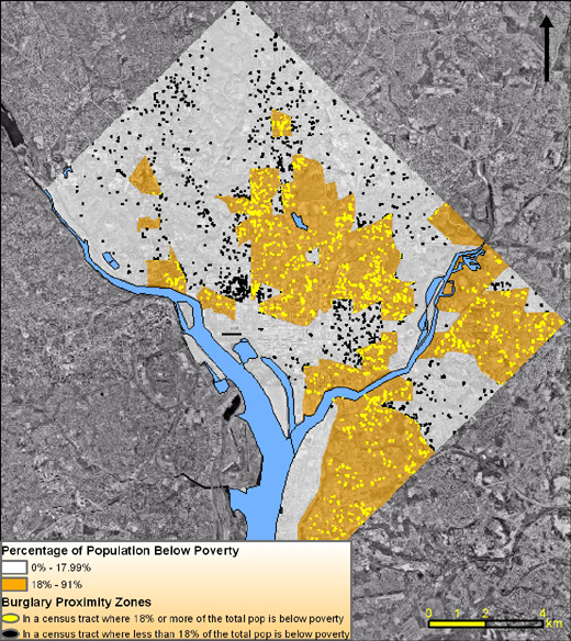
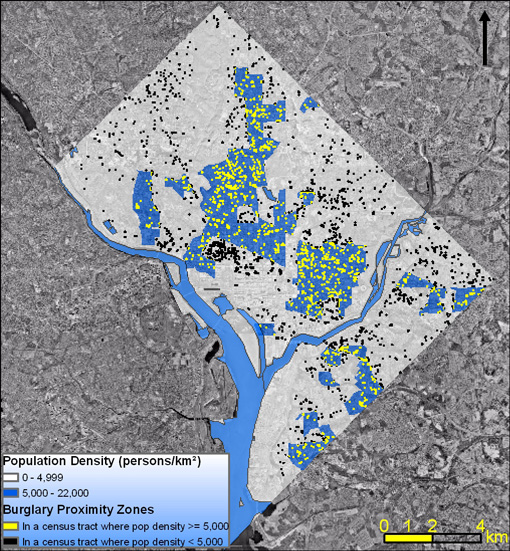
Results
CRIME FACTOR MAPS Poverty Educational Attainment Population Density
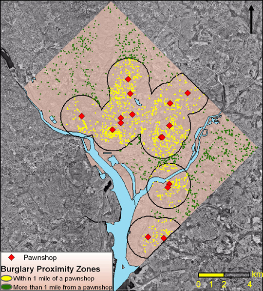
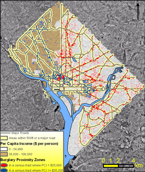
Primary Caregivers Proximity to Pawnshops Proximity to Major Roads
|
Analysis As theorized, there were fairly significant associations between burglary locations and certain socio-economic or geographic attributes. All 6 crime factor analyses produced results that followed my general expectations. For example, census tracts with a high population density had more burglaries than a simple 1:1 ratio of area-to-burglaries would predict. Whereas only 19% of Washington, D.C.’s total area has a population density equal to or greater than 5,000 persons/ km˛, 43% of the total Burglary Proximity Zone (all areas within 50 meters of a burglary) is located here. However, it quickly became clear that my analysis failed to consider several relevant issues. As I evaluated the results, I noticed that many areas of high burglary density consistently failed to show up in the areal extent of the considered socio-economic attributes. A high burglary density is evident in census tract 84, and yet this tract does not have (1) a high population density, (2) a high percentage of grandparents as primary caregivers, (3) a high percentage of adults below poverty, and (4) a high percentage of adult males who don’t have a high school degree. In fact, the total population of this tract is only 1. I did not consider the fact that burglaries are not limited to residences. Commercial burglaries often take place in areas with little or no population at all. As such, any attempt to predict areas at risk of high burglary densities must also include factors other than those relating to social characteristics. For example, proximity to major roads (or any means of “quick getaway” for a burglar, such as a subway) is a burglary factor that is not dependant on social characteristics. Because I did not have the metadata to differentiate between commercial and residential burglaries in my dataset, perhaps I could have limited my focus to census tracts with a certain population level (at the very least to tracts where the population was greater than “0”). Another concern that came forth during my analysis is my method of using Burglary Proximity Zones instead of point features. As mentioned, I chose to create a 50 meter "buffer" around each burglary location to include census tracts and their demographics in my analysis that were near certain burglaries but did not encompass them. However, there is a possibility that such a technique would force me to undervalue areas with an extremely high number of burglaries committed in extremely close proximity. For example, if 10 burglaries were committed within a very short distance from each other, a 50 meter "buffer" raster would essentially appear the same as a 50 meter "buffer" that surrounds only 1 burglary location. Finally, an issue that should be noted is the concept of crime versus the concept of burglary. Although a burglary is always a crime, a crime is not always a burglary. The FBI’s list of known crime factors is a general one, and there is little chance that each factor described is relevant to burglary. Despite this, and as discussed, the factors which I did consider were all shown to have a degree spatial correlation to burglary.
| Conclusions Though the goals of this project were modest, I feel satisfied knowing that, at least overall, the results met my expectations. I think most students have had the experience of plugging number after number into a calculator, only to see an answer on the calculator screen that is quite obviously wrong ("the speed of the bicyclist is... 2,623,872 mph?"). Ultimately, I hope to use my findings to create a predictive model for burglary. This would require further analysis, such identifying factors that affect commercial burglary locations. Additionally, I need to find an accurate method of incorporating surroundings into my model. That is, census tracts are not islands. The image conjured up by the proverbial "wrong side of the tracks" is probably not an accurate one, as it seems more likely that most areas are usually affected by what surrounds them.
| References Crime Factors. Retrieved November 6, 2003 from the Federal Bureau of Investigation Web Site: http://www.fbi.gov/ucr/cius_02/html/web/crimefactors.html Uniform Crime Reports. Retrieved November 6, 2003 from the Federal Bureau of Investigation Web site: http://www.fbi.gov/ucr/ucr.htm
| | |||||||||||||||||||||||||||

