Title Northern Spotted Owl Search
Author Melody Rae Baldwin American River College Geography 350: Data Acquisition in GIS Spring 2004 Contact Information: mbaldwi3@edd.ca.gov
Abstract Bird watching is an old and dynamic hobby. Many birders try and use current technology to assist in the pursuit of observing a specific bird species. Would Geographical Information Systems (GIS) be useful in this pursuit? Using free data a birder will be able to target specific species, map their location and remove any barrier they think may be in the way through spatial analysis.
Introduction The National Audubon Society encourages members to watch and observe birds in their environment. The members refer to themselves as birders. For an active birder living in Northern California will the GIS software be helpful targeting a specific species for observation? Can a person obtain information or data from web sites to complete a spatial analysis of this question?
Background The National Audubon’s website has the Spotted Owl on their “WatchList” (sic) for threaten species. The Spotted Owl is chocolate-chestnut brown with round oval white spots on its body while the wings and tail are dark brown with some lighter barring. The Spotted Owl (Strix occidentalis)(fig. 1) is broken into three subspecies: Northern Spotted Owl (Strix occidentalis caurina), California Spotted Owl (Strix occidentalis occidentalis), and the Mexican Owl (Strix occidentalis lucida).The California Spotted Owl lives predominately in southern California mountain ranges while the Northern Spotted Owl’s range is in the northern coastal counties of California stretching across the top of the state. The Mexican Owl can be found in New Mexico and Arizona down into Sierra Occidental in Mexico. The owl’s habitat is coniferous forest with trees in the later-seral stage (200+ years) of growth. The forest is dense creating a cooler micro climate. Their hunting patterns are to avoid clearings. They are a year around residents with little movement except during extreme weather changes.
Methods The primary goal was to answer the question could GIS assist a birder with targeting specific species. The Spotted Owl was chosen because it is a well known and documented species in Northern California. The birder, my father, expressed his criteria for this analysis in a series of telephone conversations. As a man over 75 he had some straight forward considerations. He wanted to: • Be in a designated public land area, not private land, because of the potential drug sites, • Be able to drive to a site within 2 to 3 hours of Sacramento, • Be able to hike in terrain that is not steep, and • Be in a known Spotted Owl area. The secondary goal is to experience data acquisition for a project, and the last goal was to produce a college level research paper discussing the project. The United States Department of Agriculture (USDA) Forest Service Region 5 has a variety of Northern Spotted Owl studies on their web site. The Northern Spotted Owl Activity Center published in August 2003 contains a series of polygons covering counties in Northern California. This dataset met the criteria of location, as well, as timeliness. An email to the person mentioned on the metadata and the data was delivered within a week. The next dataset for downloading was a map of California counties from the California Spatial Library (CaSIL). Before going further it was necessary to develop a shape file of the Northern California counties with the Northern Spotted Owl Activity Centers overlaid onto it. This showed that 9 counties are all that would be needed for this project. The counties are Del Norte, Glenn, Humboldt, Lake, Mendocino, Shasta, Siskiyou, Tehama, and Trinity. Using these counties focused the search for data. The next datasets that were downloaded for the project were the Major Roads and Roads for the 9 counties. The last dataset was the Ownership dataset also from the CaSIL website. The Digital Elevation Maps (DEM) are available on a variety of web sites. However, downloading the large files in the school computer lab had a variety of problems, i.e. timed out. To save time our instructor provided the United States Geological Survey (USGS) National DEM on the school network (for classroom work only). A trick that we used while in class was to set-up a shapefile as the template which we used to downloaded the DEMs. The shapefile of the area of study acted like a mask minimizing the DEM download to only the needed area.
Northern Spotted Owl fig. 1
Results At this point in the project a general review of the datasets was done. The accuracy and usability of data is a primary concern. The review revealed only a couple of problems. The Northern Spotted Owl Activity Centers extended into Oregon. This was not changed it was a small amount of data. The CaSIL Ownership data did not include a code for Private Use or Public Use. The attribute table was exported to Excel where the Public/Private Code (PU_PR) column was manually added. The coding was kept simple using 1 representing public land, 2 private land and 3 for Department of Defense. The data was then “joined” to the Ownership attribute table. This saved time by eliminating the need to manually enter the codes. It was necessary to load the County Road data into a map and decide if the roads went into a Northern Owl Activity Center. If they did not go toward an owl activity center they were eliminated by a query mask. After many attempts and visual reviews the County Roads dataset was deleted. The data would not be useful for this project. Constructing the data layers in a map is straight forward until you get an error message. Most of the maps from the CaSIL site are done in the Albers projection with the datum in NAD 1927 and the spheroid in Clarke 1866. After many hours it took another set of eyes to see that the spheroid had been left off the second map that was being loaded into ArcMap. This created a standard “Not the same Projection” message. Using ArcTools, the shapefile of the 9 counties was set up as the map for the other layers to match and the datasets were brought it in with the same projection, datum and spheroid. The pattern for adding data was repeated the same way. Add the dataset and then convert to a raster file for spatial analysis. Until the Major Roads data set, all the other data sets fit within the nine counties. The Geoprocessing wizard was used to cut the Major Roads data set to the size of the nine counties and then converted to a raster file.
Spatial Analysis The inputting and adjustment of datasets now complete. The next step was to derive more information from specific datasets. The elevation layer was converted to slope, and both the Major Roads and Northern Spotted Owl Activity Centers were converted to distance datasets. This creates a layer with a buffer type of color scheme. In Spatial Analyst the next step is called reclassify. It is the process of converting the datasets to a common scale of 1 to 10. For this customer’s analysis flat land was given a 1 and steep slope was assigned a value of 10. The closer the Spotted Owl activity center polygon was to the road then the closer to a value of 1. The last reclassification was done on the major roads. The zone close to the road was given a value of 1. This leaves you with a variety of colorful maps that are disconnected. This is when the datasets are given a weight by the percentage assigned and then combined back together as one map. The public land was assigned fifty percent because of the safety issue. Then low slope or flat land was given twenty-five percent. This left the distance from the road and the distance to the owl activity center both weighed at twelve and a half percent. Using the Raster Calculator the weights were entered and the result is one map.
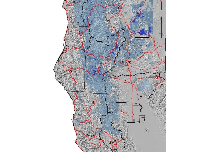
Northern Spotted Owl Sighting Map fig. 2
Conclusions The final map shows the best areas for observing a Northern Spotted Owl (fig. 2). The map will be given to the requester, Dad, along with this report for his trip over Memorial Day weekend. He will be able to use the map in his pursuit of a specific species of bird. He will not have to hike up any steep hills or far from the road. The project did answer the original question presented within the criteria developed. The project also revealed other things during the process. As a novice map maker the Spatial Analyst maps are not very good looking. The attraction of choosing this career field was the idea of creating a map that was interesting and revealed a lot of information for the reader to analysis and discover. For many readers, the National Geographic maps come to mind when thinking of colorful useful maps. This question then led to more experimentation and exploring. How do you make an acceptable raster map look “prettier?” What is prettier? This led to experimenting with hill shade, colors and masking data. Then experimenting lead to a lot of exploring and learning. The details of that part of the project have been left out of this paper. One lesson that will be shared with you is, if you are considering a future map project, double your allocated time line for the project. Between downloading, reviewing, experimenting and plain getting lost the project took three times longer than originally planned. Yet that time spent will be useful for any GIS Analyst or GIS want-to-be as their knowledge and experience grows. The class project was defined so that the student was forced to think, create and solve questions as they worked through the process. Many of the ESRI tutorials are set up to be followed step by step in a general recipe style of teaching or learning. The recipe approach is necessary for the first few maps. It was rewarding to develop an original map with data that was of interest to the author.
References California Spatial Library: California Department of Forest and Fire Protection. County Boundaries (1:24000). Available http://gis.ca.gov/meta.epl?oid=21384 [2004 April 15]. California Spatial Library: Teale GIS Solutions Group. Major Roads. 1997 Available http://gis.ca.gov/meta.epl?oid=267 [2004 April 15] California Spatial Library: United States Geological Survey (USGS) Digital Line Graphic (DLG) transportation. Roads. Available http://casil-mirror1.ceres.ca.gov/casil/gis.ca.gov/teale/roads/ [2004 April 15] Counties: Del Norte, Glenn, Humboldt, Lake, Mendocino, Shasta, Siskiyou, Tehama, Trinity California Spatial Library: Teale GIS Solutions Group Public Land Survey System Available http://gis.ca.gov/meta.epl?oid=298blic [2004 April 15] California Spatial Library: Teale GIS Solutions Group. United States Geological Survey (USGS) National Map Digital Elevation Map Available http://gis.ca.gov/meta.epl?oid=277 [2004 April 15] Gutierrez, R.J.; Franklin, A.B.; Lahaye, W.S. 1995. Spotted Owl (Strix occidentalis). The Birds of North America, No. 179 (A. Poole and F. Gill, eds.). The Academy of Natural Sciences, Philadelphia, PA, and The American Ornithologists' Union, Washington, D. C. Lily, Douglas Using Christmas Bird Count Data in GIS Available http://ic.arc.losrios.edu/~veiszep/call.htm [2004 April 15] National Audubon Society, Inc. Audubon WatchList 2002. Available http://audubon2.org/webapp/watchlist/viewWatchlist.jsp [2004 April 15] United States Department of Agriculture (USDA) Forest Service. GIS Clearinghouse. 2003. GIS Clearinghouse – Region 5 Available http://www.fs.fed.us/r5/rsl/clearinghouse/gis-download.shtml [2004 April 15].