| Title Plant Communities of the Putah Creek Watershed | |
|
Author Leah Gardner Miller American River College Geography 350: Data Acquisition for GIS Fall 2004 Contact Information: Leah_M@pacbell.net | |
|
Abstract The Putah Creek watershed, with its varied topography and rainfall, hosts a variety of plant communities. In prepartaion for an upcoming project mapping riparian vegetation along the creek, a base map of the watershed is needed. Existing secondary data can be used since analysis will not be carried out on the basemap itself. | |
|
Introduction The vegetation/land cover data comes from the California Gap Analysis Project, UC Santa Barbara and USGS. This is a widely used dataset at a scale of 1:100,000. It can be downloaded from Casil (California Spatial Information Library) or from the UC Santa Barbara biogeography website. The watershed outline comes from the California Interagency Watershed Map of 1999 from Casil or the NRCS CalWater website. It is a hierarchical system of six nested levels and I will use the top 2 levels: Hydrological Region (HR) and Hydrological Unit (HU). | |
|
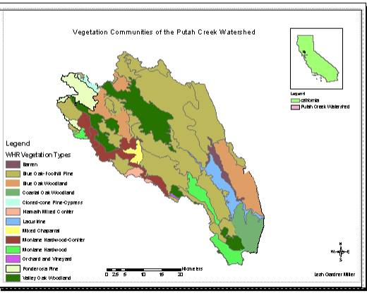
Background The Putah Creek watershed encompasses 810 square miles including parts of Napa, Lake, Yolo, and Solano counties. Elevations range from sea level to nearly 5,000 feet and annual rainfall averages from 17 to over 60 inches. This leads to a high diversity of plant species and plant community types in the watershed. The vegetation data from GAP uses the CWHR (California Wildlife Habitat Relationships) system of classification. The community mapping is at a coarse scale for generalized landscape characterization and the Data Dictionary in the GAP website warns that "because source information ranged widely in date and reliablilty, the current database is uneven in both level of detail and accuracy." | |
|
Methods After downloading the two datasets, several steps were necessary to process the data, using WinZip and ArcGIS, to make them useful for my project. From the Gap Analysis Project website, I downloaded by region choosing the northwestern California region and clicking "Export". This gave me a zipped file titled "landcov.e00.gz" which had to be extracted using WinZip. The resulting "nwveg.e00", an interchange file, had to be processed further using ArcToolbox. In Conversion Tools, I choose "Import to Coverage" and "Import from Interchange file", resulting in "nwveg", which had to be exported from coverage to shapefile to finally get "nwveg.shp". The last step was to convert the shapefile to the correct coordinate system. In ArcToolbox Data Management Tools, I used Projections>Project Wizard to select UTM zone 10 as the coordinate system. The next dataset for downloading was the watershed map from CalWater, choosing the Sacramento River watershed, Region 5. But since my goal was to get a smaller hydrological unit (HU) within this hydrological region (HR), several steps in ArcGIS were necessary. From the Selection menu, I used Select by Attribute, choosing "cwreg5". Next, I choose the field "HUNAME", hit the = button on the calculator, and from the complete list, choose Putah Creek. The resulting query statement read "HUNAME = PUTAH CREEK." Going back to the table of contents and right clicking "cwreg5", I choose "Export Data - Selected Features" and named the new layer "putah-watershed.shp". I then had to use Dissolve in the Geoprocessing Wizard to get rid of the extraneous details, since I only needed the outline of the watershed. I choose "putah-watershed.shp" as the layer to dissolve and the field "HUNAME" to dissolve on. This finally resulted in a boundary for the desired watershed, which I named "putah_boundary.shp" and gave the layer a clear fill and thickened line. The two datasets were finally ready to combine. Using the Geoprocessing Wizard Clip funtion, I choose "nwveg" as the layer to clip and "putah_boundary" as the clip layer. The clip layer acts like a cookie cutter on the other layer so my result showed the vegetation for the area within the watershed boundary, named "putah_veg.shp." The final steps involved cartographic design principles. Clicking on the layer properties and choosing "Properties" "Symbology", then going to "Categories> Unique Values>Add all Values" allowed all the plant community types to be displayed on the map. I had to spell out the abbreviated vegetation names and experiment with the color palletes. Then, going to layout view, I added in a title, legend, north arrow, scale bar, and my name to get a properly finished map. | |
 | |
|
Results The resulting map provides
an easy to see generalized representation of the plant communites of the
watershed. Blue Oak-Foothill Pine Woodland covers the greatest area, with
Valley Oak Woodland as the second dominant type, which seems to be
realistic from my experience driving around the area. However, chaparral
seems to be underrepresented. This may reflect the level of inaccuracy of
the dataset at this scale or recent land use changes, including fires.
| |
 | |
|
Conclusions From this project, I
learned that data acquisition itself is fairly easy. There is an abundance
of available free data. However, accessing the accuracy and
appropriateness of the data is extremely important. Making the data useful
for your particular project is the difficult and time-consuming part of
the process. Many of the tools in ArcToolbox are useful. Using a flowchart
can help to organize the steps necessary and the order in which the steps
need to be done, as well as to graphically communicate your process to
others. | |
|
References California Spatial Library. http://gis.ca.gov. CalWater: California Interagency Watershed Map of 1999. Available at http://www.ca.nrcs.usda.gov/features/calwater California Gap Analysis Project. Available at http://www.biogeog.ucsb.edu/projects/gap/gap_proj.html Barbour, Michael G. and V. Whitworth, 2000. Vegetation of the Putah-Cache in A Thinking Mammal's Guide to the Putah-Cache Bioregion. University of California, Davis. Mayer, Kenneth E. and W.F. Laudenslayer, 1988. A Guide to Wildlife Habitats of California California Department of Fish and Game, Sacramento. Ormsby, Tom, E. Napolean, R. Burke, D. Groess, and L. Feaster, 2001. Getting to Know ArcGIS ESRI Press, Redlands. | |