| Volume Calulations with 3D Analyst | |
|
Author Karen Miller American River College Geography 350: Data Acquisition in GIS Spring 2007 | |
|
Abstract GIS is more than just a map or cartography tool. It can be used for sophisticated analysis and data acquisition. This project demonstrates ArcGIS capabilities for volume calculations and 3D modeling of a proposed dam and reservoir. Also emphasized is the workflow process of deriving the data required, obstacles met and overcome, and the final product reached. | |
|
Introduction It is not uncommon for the GIS user to face the question of "how do I get there from here" in everyday projects. That is, how do you achieve a desired result with the data you have been provided? Here, as a project progresses, unexpected events occur and new problems are encountered, which requires the GIS user not only be a good problem solver, but also as flexible as the software itself. This project will illustrate one such experience I have had and show how often times, there is a learning curve to be overcome during said process. As part of a Fatal Flaws Analysis for a proposed dam, both the alignment and height of the dam must be analyzed in order to produce an area-capacity curve. This project will use ArcGIS 9.2, Spatial Analyst, and 3D Analyst to create an elevation surface and calculate areas and volumes of the proposed reservoir. The general approach will be focused based on the particular data provided - a CAD file of contours at a 5 foot interval, and basic information about the proposed dam (crest elevation and slope on either side) and to examine various methods for creating the new data, i.e. an elevation grid and area and volume calculations. | |
|
Background Although GIS has not historically been at the forefront of 3D modeling and visualization, recent releases of ESRI's ArcGIS and 3D Analyst Extension have made great strides in the 3D direction. In addition to the tasks demonstrated here, 3D Analyst includes a number of other tools for working with data in 3D, including ArcScene, the 3D companion to ArcMap. Noteworthy is the fact that these references to "3D" are not technically 3D. Instead, we refer to this type of GIS data as 2.5D. This is because the GIS only allows one "z" value for every "x,y". This is why data is often refered to as a "surface". What is below that surface is not usually modeled in the GIS for this reason. Perhaps this is one of the major limitations of "3D" modeling using ArcGIS products. For the purposes of this project, volume (which definitely is a true 3 dimensional measurement) can be calculated by intersecting a plane at a specified height with the input surface. | |
|
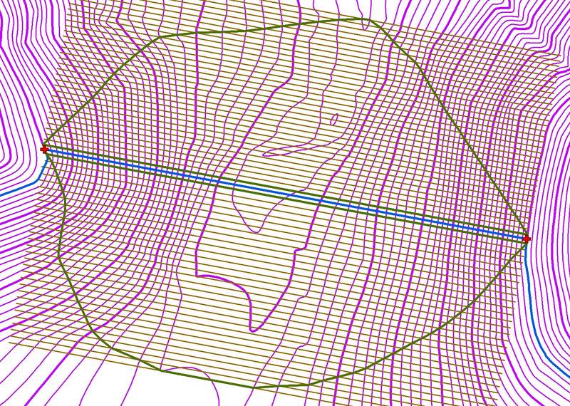
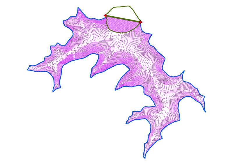
Methods
| |
 |  |
|
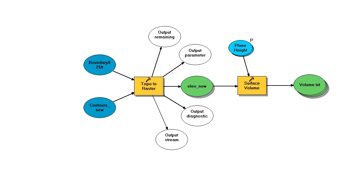
Model Builder
| |
|
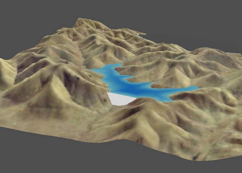
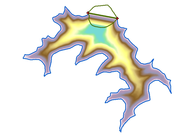
But wait, isn't there anything pretty to look at?
|
|
|
Results Even with a few bumps along the way, this project resulted in volume calculations for the capacity of the proposed reservoir at an interval of 10 feet, measured in acre-feet. This could easily be applied to a capacity curve for a visual describing how much water could be stored as a result of the building of the proposed dam. The process of making these calulations led their way into the creation of a 3D model of the project area, which likely will be seen on the report cover submitted to the client. | |
|
Analysis This project proved to be quite a learning experience and problem solving exercise. I had never done anything like this before, and as a result, I met with some challenges I didn't expect. Determining which tools I needed to use required a refresher's look at the help system, but even so, the output was still not exactly what I wanted when I used the Topo to Raster tool. It is helpful to know not only what tools are available, but the basics about how they derive their output. All in all, I was able to work through the problems and find solutions, and my final product was exactly what was needed. Model Builder came in very handy. After my initial volume calculations, I was asked to perform this task again, as the crest elevation was going to change. The model I created allowed me to run the same processes over again with new imputs very easily. | |
|
Conclusions This project has succesfully shown that GIS is more than just a map or cartography tool. Although underutilized in many businesses and even industries, the possibilities are endless so long as the GIS user is ready to stretch his/her mind. It can be used for numerous types of data acquisition and analysis, including but by no means limited to what has been shown here. The key is education, not only on how to do these things, but more importantly, what types of things can be done. This is the starting point from which all such projects begin. It is important for the GIS user not to be afraid of trying new things. Although, I had never done a project quite like this, I certainly did use it to learn as much as possible. Next time something similar comes up, I will be much more prepared and efficient at solving the problem at hand. | |
|
References Environmental Systems Research Institue (ESRI), 1999-2006. ArcGIS Desktop Help. | |