This project relies upon established methodologies using ESRI Spatial Analyst extension tools and Model Builder in ArcMap to generate a least cost path for proposed transmission lines. There have been several academic studies targeting the use of GIS analyses for energy development. The main concept for this paper is based upon two main sources: 1) Andrew Schmidt's paper (cited below), which uses raster data to model transmission routing; and 2) Professor Hugh Howard's working LCBF model (cited below) for gas transmission siting.
Additionally, The Joint Institute for Strategic Energy Analysis (JISEA or Joint Institute), which was created by the Alliance for Sustainable Energy, the National Renewable Energy Laboratory (NREL), the Massachusetts Institute of Technology (MIT), Stanford University, University of Colorado-Boulder (CU), Colorado School of Mines (CSM), and Colorado State University (CSU) has been exploring potential open source GIS siting tools for use by renewable energy developers and have posted a concept paper, A GIS-Based Mapping and Optimization Tool to Aid Siting, Design, and Assessment of Utility-Scale Energy Development , which is intended to "...provide a mechanism to comprehensively evaluate a proposed energy project, or select a site for a new energy project... [T]his tool will be effective for stakeholders with varying degrees of preference for economic considerations and environmental effects. A first application of this tool will be siting of potential future large scale solar thermal plants." Since there has been such an enormous emphasis placed on the development of renewable energy resources, the federal government has devoted millions of dollars in funding to advance GIS tool development and make them available to developers. One such example is the SunShot Initiative , a Department of Energy (DOE) program designed to decrease the overall costs of solar energy systems.
While both the Joint Institute and Sunshot programs seek to develop generation siting tools, the concepts and mehtodologies employed are very similar to those used for a LCBF path tool for high voltage transmission lines and were useful in this study.
Data Search -
Elevation data: National Elevation Dataset (NED) The National Map Seamless Server
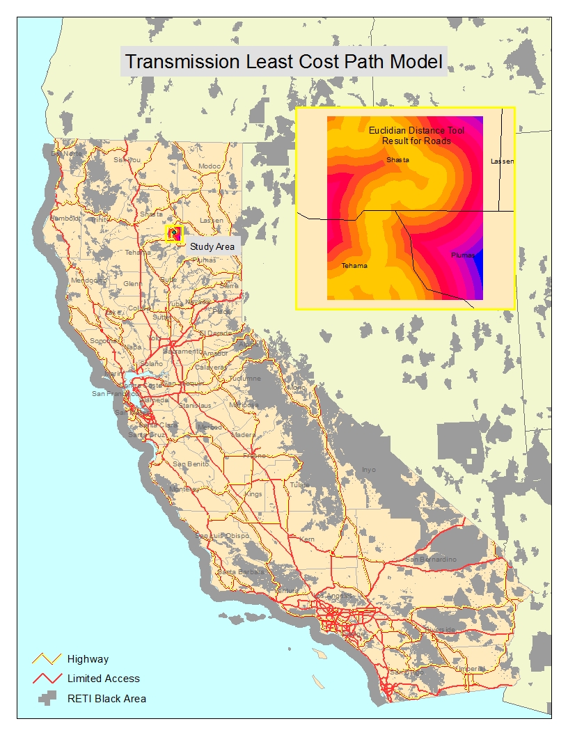
Environmental Conflict Data: Renewable Energy Transmission Initiative (RETI)
ESRI Data: Major Roads
Data Selection -
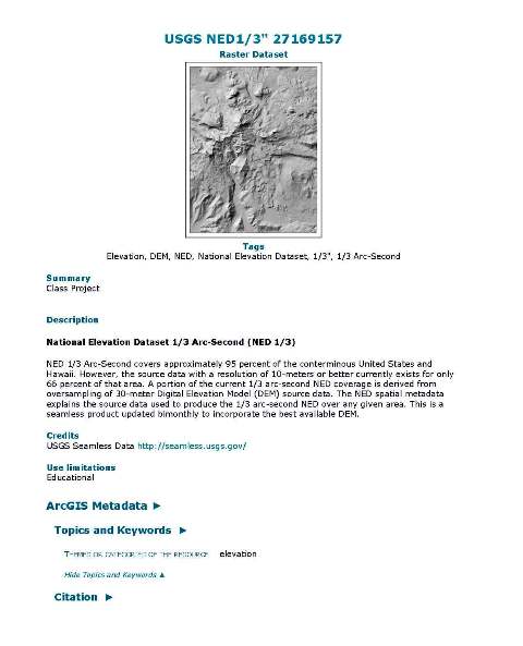
The NED 1/3 Arc-Second (#27169157) was chosen because it was granular enough (10 meter resolution) and covered an area in northern California sufficient for this proof of concept model. The NED spatial metadata explains the source data used to produce the 1/3 arc-second NED. The NED description indicates that the resolution of the raster data is 10 meters; upon inspection of the metadata, it is actually slightly better - 9.3 meter (rounded) resolution.
RETI Conflict Data was chosen because it aggregates all known sensitive lands into one shapefile. Conflict areas include: Designated Federal Wilderness Areas, Private preserves of The Wildlands Conservancy, Wilderness Study Areas, National Wildlife Refuges, Units of National Park System (National Parks, National Monuments, National Recreation Areas, National Historic Sites, National Historic Parks, National Preserves), Existing Conservation Mitigation banks under conservation easement approved by the state Department of Fish and Game, U.S. Fish and Wildlife Service or Army Corps of Engineers, Inventoried Roadless Areas on USFS national forests, CA state defined wetlands, National Historic and National Scenic Trails, CA State Wilderness Areas, National Wild, Scenic and Recreational Rivers, CA State Parks, BLM King Range Conservation Area, Black Rock-High Rock National Conservation Area, and Headwaters Forest Reserve, DFG Wildlife Areas and Ecological Reserves, BLM National Recreation Areas, BLM National Monuments, Lands precluded by development under Habitat Conservation Plans and Natural Community Conservation Plans, Lands specified as of May 1, 2008 in Proposed Wilderness Bills (S. 493, H.R.3682), Military Bases, Urban Areas, Schools, and other related sensitive areas.
ESRI Major Roads dataset was chosen because it covered the area of interest.
Data Processing-
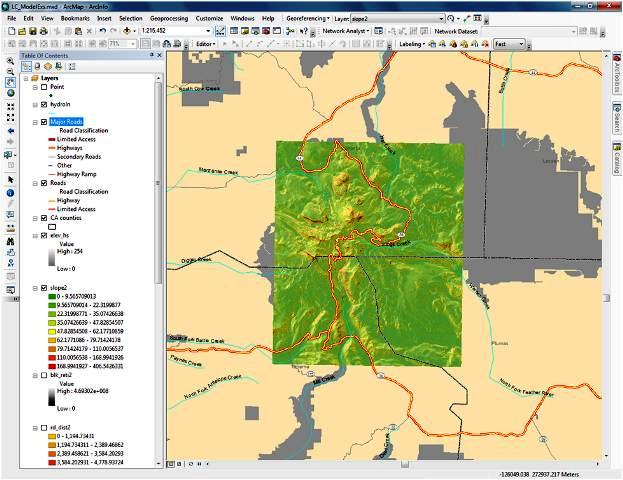
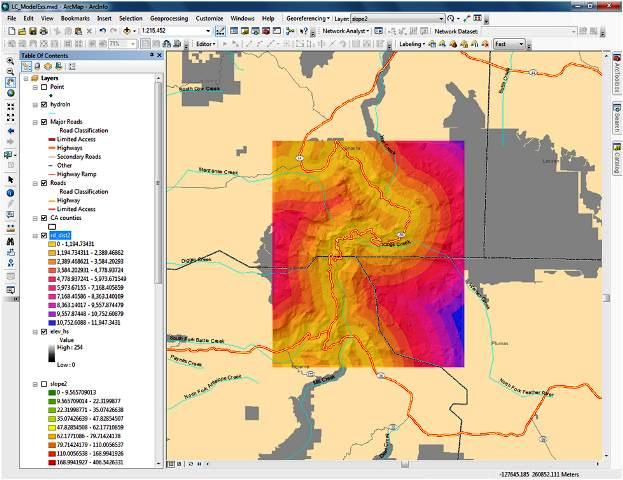
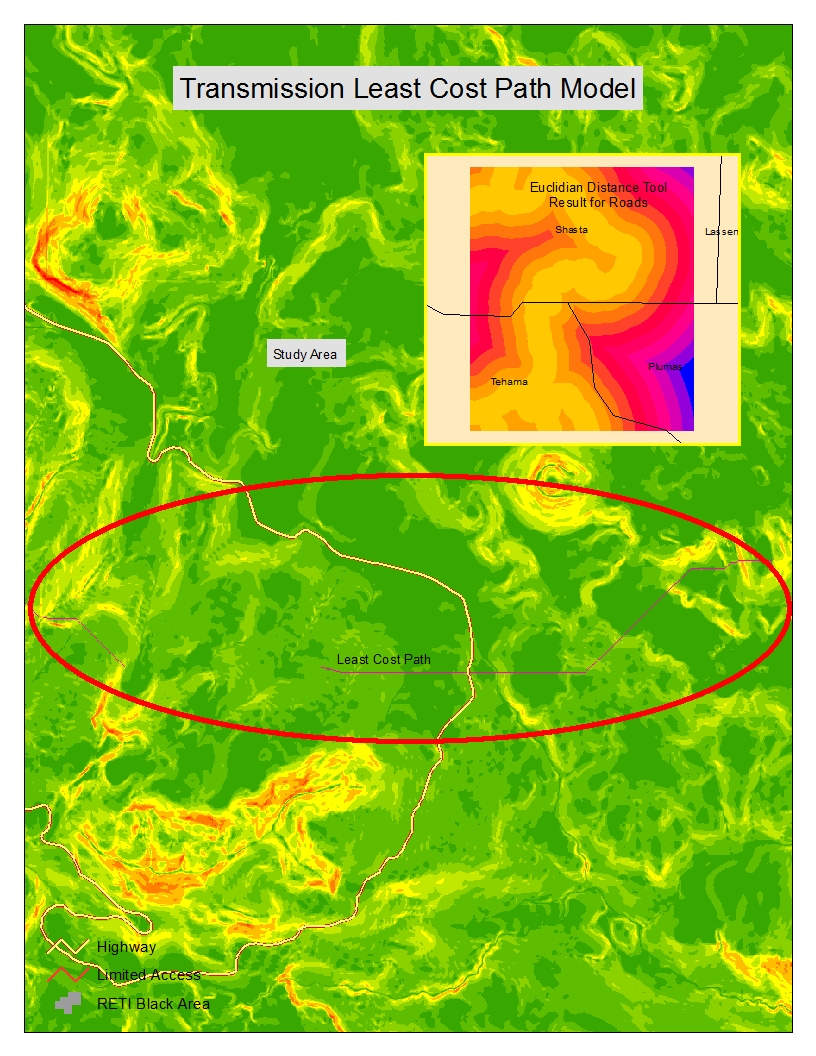
All data was projected to California Teale Albers (North American Datum 1983). Datum transformations were incorporated during projection when applicable. All data outputs during model runs were clipped to the extent of the elevation raster. The slope raster (Figure 3) was derived from the NED raster, and the roads distance raster (Figure 4) was created using ESRI Major Roads vector data as the input to the Euclidean Distance tool. The RETI Blackout vector data was converted to a raster using the feature to raster tool.
Metadata Creation
Metadata was created for the unique datasets acquired/created for the project - RETI Blackout, Euclidean Road Distance, Slope and the elevation raster acquired from the USGS Seamless Data Warehouse - Figure 5 below shows an example of the output from ArcCatalog.
Model Construction -
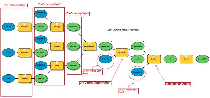
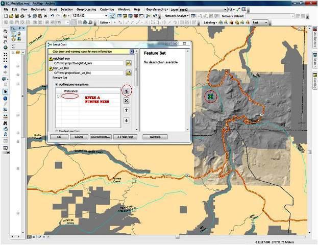
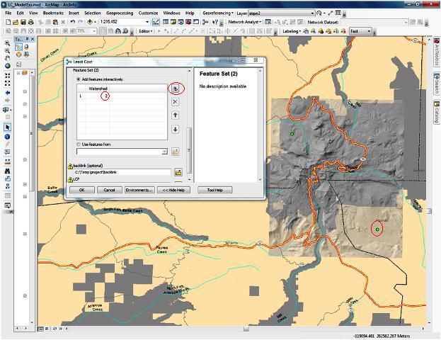
The model (Figure 6) uses raster data - elevation, slope, social, environmental and cultural data (RETI Blackout areas), each reclassified and assigned cost values for each pixel as input and computational values. A start and end point are interacively chosen by the user in an ArcMap session and are then connected using complex algorithms to follow the path of least resistance (cost), so-to-speak. These digital values and direction-distance data determine optimal path, which is output as a raster and can then be converted to vector (line) data. Figure 5 below demonstrates the formation of a least cost path using Model Builder and the major model components are identified (first the beginning and end points that are interactively selected by the user are set (feature sets that are circled in red)): 1) In the first pre-processing step, the slope, road distance and RETI Blackout rasters are reclassified into 10 equal interval classes; 2) the reclassed rasters are given a weighted importance (in percentages) - these values are parameters and can be changed by the user; 3) the weighted rasters are combined using the raster calculator to create a single weighted raster; 4) the Cost Distance tool performs its algorithmic calculation - the least accumulative cost distance for each cell to the nearest source over a cost surface; 5) the Cost Path tool creates a rasterized path between the beginning and end points (the back link input defines the neighboring cell (pixel) that is the next cell on the least accumulative cost path to the nearest source); and 6) the rasterized pixels are then expanded for a better visual line effect.
The model parameters and logic are correct; however as stated above, some data error sporadically stops the model during the execution of the Cost Distance tool. If more time were available, perhaps a solution could be found via the ESRI support center or another GIS professional.