Urban Growth in Sacramento County from 2002–2011
Joanna Nishimura
American River College: Geography 350
Data Acquisition, Fall 2012
Abstract
Given current population projections, minimizing the impact of rapid urban expansion will be one of the greatest and most important environmental challenges of the 21st century. In this project, the author attempts to use remotely sensed data to assess urban land cover expansion between 2002 and 2011. LANDSAT 4-5 TM imagery (30-meter resolution) captured in 2002 and 2011 was used to run a basic unsupervised classification of Sacramento County using the Image Classification tool in ArcGIS. Between 2002 and 2011, a 5.2% decrease in water coverage, 3.1% increase in urban coverage, and a 2% increase in vegetation coverage were observed. Based on visual observations, the majority of urban growth occurred in the southern and central portions of Sacramento County. Unfortunately, an accuracy assessment was not performed, which makes it difficult to quantitatively to evaluate the results of this study.
Introduction
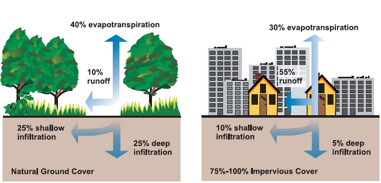
As of 2008, half of the world's population (over 3.2 billion people) lived in urban centers and by 2030, urban centers will support over 5.0 billion people [United Nations 2005]. Minimizing the impact of this rapid urban growth will be one of the greatest and most important environmental challenges of the 21st century. Currently, Sacramento County has a population of approximately 1.4 million, making it the 8th most populous county in the state and the 25th in the US [US Census Bureau 2011]. The last major housing boom in Sacramento resulted in the widespread conversion of farmland to housing developments. This rapid urbanization results in the replacement of natural land cover with impervious surfaces such as roads, houses, buildings, and parking lots. These impervious surfaces prevent the infiltration of water and negatively affect local hydrology, geomorphology, and the health of watershed ecosystems [Konrad 2003]. This project uses the Image Classification tool in ArcGIS to assess increases in urban land cover between January 2002 and February 2011 in Sacramento County.
Background
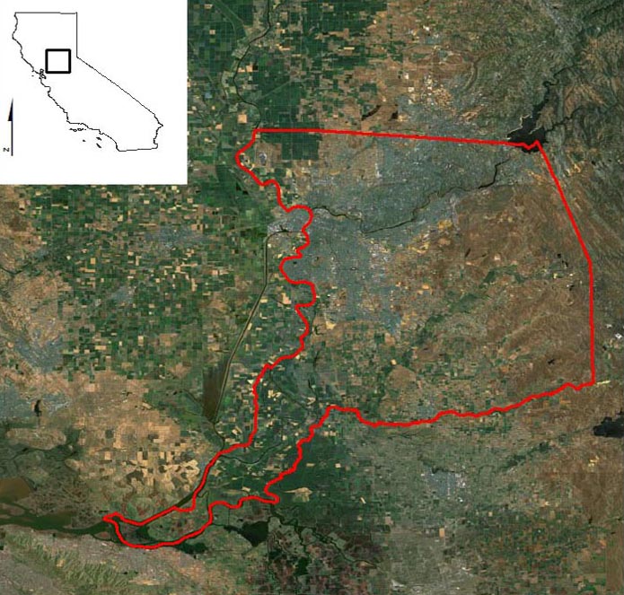
Sacramento County is approximately 994 square miles, of which 97% is land and 3% is water [US Census Bureau]. The geographical location of the county and the aging levee system leave Sacramento County particularly vulnerable to flooding. The widespread conversion of agricultural land to housing developments has greatly increased the amount of impervious surface and the risk of urban flooding. Understanding population growth in Sacramento County, proper urban planning, and reducing the amount of impervious surface coverage is key in preventing urban flooding and future human and property loss.
Housing developments generally contain anywhere between 20-85% impervious surface coverage and scientific studies have determined that watershed ecosystem health declines at 10-15% impervious surface coverage [Brabec et al. 2002]. In urban settings, the vast majority of land covers like streets, sidewalks, and rooftops are impervious to water infiltration. Impervious land covers increase the rapidity of urban runoff while also decreasing the potential storage capacity of a given area [Konrad 2003]. During storm events, impervious surfaces become quickly saturated with water, resulting in a higher degree of urban runoff [Konrad 2003]. Streets, gutters, and drains efficiently channel urban runoff to ditches and streams, resulting in a higher peak discharge rate than would normally occur in an unaltered environment [Konrad 2003].
Urban land cover data can be used to monitor population growth, create urban development models, or identify areas where impervious surfaces may significantly contribute to urban flooding. Historically, impervious surface mapping has been conducted through field surveys and using handheld global positioning systems (GPS) to mark boundaries of different land covers [Weng 2012]. This method, while extremely accurate, is time consuming and expensive [Weng 2012]. More recently, the use of remotely sensed data has provided a cheaper and more efficient method to map land cover [Weng 2012]. Satellite or aerial imagery is acquired, scanned, and different land covers are identified by feature extraction algorithms in a process called image classification [Weng 2012]. Image classification categorizes an image based on spectral classes of individual pixels or groups of pixels [Weng 2012]. While this method can produce less reliable results, feature extraction algorithms are continuously being refined to provide more accurate results [Weng 2012].
Methods
Two sets of LANDSAT 4-5 TM images of Sacramento County, were used for this project. Each image has a 30-meter resolution and was downloaded from USGS Glovis [glovis.usgs.gov/]. Image sets contained <10% cloud cover and were captured in January 2002 and February 2011 when obstruction from foliage would be at a minimum. When downloaded from USGS Glovis, each image consisted of seven individual .tif files representing different satellite sensor bands. Each image set was composited into a traditional false color composite image consisting of Band 4 (red), Band 3 (green), and Band 2 (blue). In this band composition, healthy vegetation will appear red, densely populated urban areas are blue, and bare earth areas are dark to light brown.
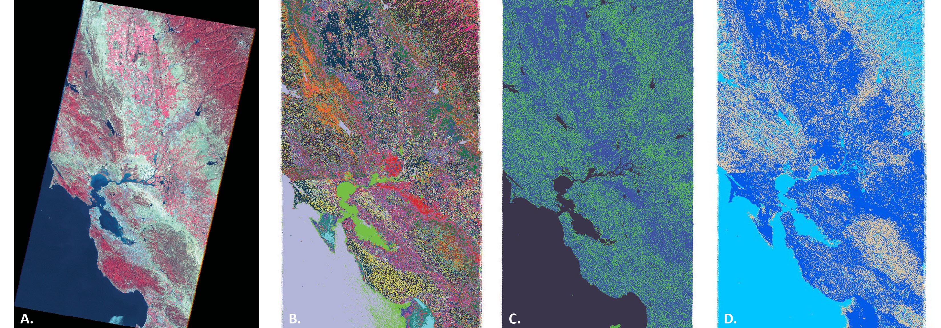
After the band compositing, the black borders (null values) were clipped by adding each image to a raster dataset, mosaicking the image, and excluding null values. The image classification toolbar was activated and an Iso Cluster Unsupervised Classification was run on each image. Even though I wanted the end product to be segmented based on three distinct land covers (urban, vegetation, and water), I specified the unsupervised classification to have 20 classes with a minimum class size of 50 and a sample interval of 10. This initial classification was saved as a new output file and I manually checked the validity of each of the 20 classes against the original unclassified satellite imagery by using the Swipe Tool in the Effects Toolbar. All 20 classes were designated as either urban, vegetation, or water and the results were then reclassified to an appropriate color scheme. The final reclassified classification was then clipped to a border of Sacramento County downloaded from the Sacramento Council of Governments [sacog.org].
Results
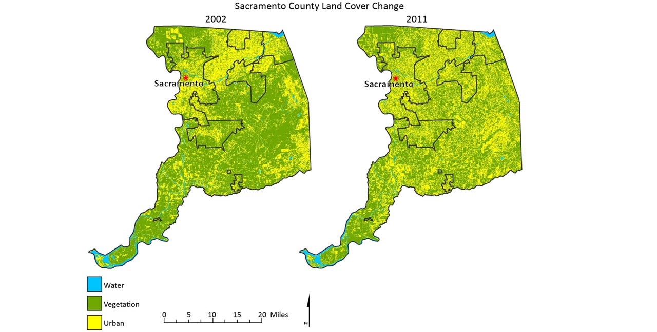
Between 2002 and 2011, there was a 3.1% increase (30.1 square miles) in urban land cover, 5.2% decrease (49.5 square miles) in water cover, and a 2% increase (19.4 square miles) in vegetation cover.
| 2002 | ||
|---|---|---|
| Land Cover Class | % of Sacramento County | Area (square miles) |
| Water | 26.9 | 259.2 |
| Urban | 27.3 | 263.4 |
| Vegetation | 45.8 | 442.1 |
| 2011 | ||
|---|---|---|
| Land Cover Class | % of Sacramento County | Area (square miles) |
| Water | 21.7 | 209.7 |
| Urban | 30.4 | 293.5 |
| Vegetation | 47.8 | 461.5 |
Analysis and Conclusion
The results showed an increase in urban and vegetation cover while a decrease in water coverage between 2002 and 2011. The increase in vegetation and decrease in water coverage were unexpected results. The decrease in water coverage between 2002 and 2011 could reflect a decrease in river and water body size, but likely resulted from inaccuracies inherent in the image classification process. It appears that more urban growth occurred in the southern and southeastern portions of the county and that in general, urban cover in the central regions becomes sparser. No accuracy assessment was performed, so it is difficult to evaluate the validity of the image classification.
Feature extraction algorithms work by assigning land cover classifications to pixels based on the unique spectral signature of each pixel. The Iso Cluster Unsupervised Classification tool in ArcGIS provides a quick and easy method to classify an image without extensive prior knowledge of the actual land cover. However, unsupervised classifications rely exclusively on the spectral classes of individual pixels. In most cases, land cover classes represent a wide range of spectral classes and may not produce accurate results. Without conducting an accuracy assessment, which would compare ground-truthed land cover classes as determined by field surveys to image classification results, it is difficult to evaluate the validity of these results. Given the time constraints of this project, conducting a field survey and subsequent accuracy assessment were unrealistic.
The relatively low resolution (30-meter) of the LANDSAT 4-5 TM imagery means that each pixel most likely represents multiple land covers. One pixel represents approximately 1/10 of a city block. If the city block is partially obscured by tree canopy, it is likely that the pixels may be completely classified as vegetation, instead of a mixture of vegetation and urban cover. This problem was particularly apparent in the midtown and downtown regions in Sacramento County. In the classified images, the gridwork system of roads is barely recognizable because of the dense tree canopy. Large portions of these regions were misclassified and urban cover is greatly underrepresented in these areas. This problem could be remedied by using higher resolution satellite imagery like Geo-Eye, Quickbird, or WorldView; however, most of this imagery is either restricted access or is fee based.
Overall, I thought that the Iso Cluster Unsupervised Classification tool in ArcGIS performed was an easy-to-use tool that provided average to below average results. The poor satellite imagery resolution likely added to the inaccuracy of the results and I would hesitate at using unsupervised classifications when attempting to map a relatively small area. In the future, I would conduct a supervised or hybrid classification, which uses training sites of known land cover type in order to create a more accurate classification algorithm.
References
Brabec, E., Schulte, S., and Richards, P. 2002. Impervious Surfaces and Water Quality: A Review of Current Literature and Its Implications for Watershed Planning. Journal of Planning Literature, 16:499-514.
Department of Economic and Social Affairs: Population Division. 2005. Population Challenges and Development Goals. United Nations: 1-57.
Konrad, C. P. 2003. Effects of Urban Development on Floods. USGS Fact Sheet, 076(03):1-4.
NEMO Photo Gallery. Nevada Cooperative Extension. http://www.unce.unr.edu/programs/sites/nemo.
Sacramento County, California, 2011. State and County QuickFacts. United States Census Bureau, http://quickfacts.census.gov/qfd/states/06/06067.html.
Urban Nonpoint Source Fact Sheet. 2003. EPA Fact Sheet, EPA 841-F-03-003. water.epa.gov
Weng, Q. 2012. Remote Sensing of Impervious Surface in the Urban Areas: Requirements, Methods, and Trends. Remote Sensing of Environment, 117: 34-49.