Debris Flow Hazard Mapping with GIS:
Preliminary Exploration of Issues
Theodore C. Smith
American River College, Geography 350: Data Acquisition in GIS; Winter 2012
7053 Enright Drive, Citrus Heights, CA 95621
Abstract
Strom-triggered debris flows are a significant hazard in various parts of the
world.
Introduction
This project was undertaken to demonstrate proficiency in acquiring and generating
GIS data. The selected project is related to my geology expertise but should
not be used for site-specific design and construction.
Background
In about 1976, I developed a model debris flow hazard map for a four square
mile area of the Montara Mountain Quadrangle between the City of Pacifica and
the community of Montara. The model was developed by interpreting several vintages
of aerial photographs to identify areas exceeding 20% slope with convex upward
curvature. [See Smith (1988) for a more complete description of the methodology.]
The initial analysis was completed by hand and eye, requiring days to weeks
to complete. The results were presented at a meeting of the Geological Society
of America (Smith, 1977). Note that all of the hillslopes in the study area
are underlain by rock units that produce sandy soil.
During a 32-hour period on January 3-5, 1982, a major rainstorm triggered about
85 debris flows in the study area, presenting an opportunity to review and refine
the method (Smith, 1988). Those results suggested that the methodology was valid
and might be useful for mapping mudslide hazards as part of the National Flood
Insurance Program. However, unlike 100-year flood zone maps, the method relied
heavily on the interpretive abilities of individual scientists. Unless a way
could be found to standardize the map creation process, adoption was unlikely.
Within a few years, staff at the US Geological Survey began experimenting with
a GIS version of the analysis. However, only one arcsecond (~30 m resolution)
data and limited GIS programs were available. Earl Brabb (personal communication,
about 1990) noted that those data sets were created by cartographers who, because
of high production rate requirements, inadvertently introduced errors in the
data that were difficult to detect and correct. First attempts to standardize
the process were somewhat disappointing. Although small-scale susceptibility
zone maps were produced for the San Francisco Bay region, the small-scale landslide
maps coupled with the limited resolution GIS data resulted in only 82% of debris
flow sources aligning with the most likely source zones in the calibration areas
and 53% in the entire bay region (Ellen et al., 1997).
Today, one-third arcsecond (~10 m) data are available.
This project digitizes one of the Smith (1977) maps and qualitatively compares
a GIS model using elevation data and ArcGIS 10.
Methods
Steps in this project were as follows:
- 1. Visit http:// http://store.usgs.gov/
- Searched for Montara Mountain 7.5-minute quadrangle images. Available
map images include 1949, 1956, 1993, 1997, and 2012 (in two parts).
- Downloaded 1956 map (gda_5682919.zip)
- Downloaded 1993 map (gda_5682933.zip)
- Visited USGS Earth Explorer
- Searched for Montara Mountain 7.5-minute quadrangle scanned map
- Downloaded o37122e4.tgz
- Unzipped files (o37122e4.fgd, o37122e4.tfw, o37122e4.tif)
- 3. Create new ArcGIS file
- Add Montara Mountain 7.5-minute quadrangle map
- Check coordinate system data (NAD 27 UTM zone 10N)
- Photograph paper maps from Smith (1988); import images into ArcGIS; register images, and
digitize debris flow data.
- Zoom in to visually inspect accuracy. Evaluate qualitatively.
- Obtain 1 ArcSec and 1/3 ArcSec elevation data from USGS.
- Add elevation data to ArcGIS; create hillshade and curvature maps.
- Compare hillshade and curvature maps and evaluate qualitatively.
Results
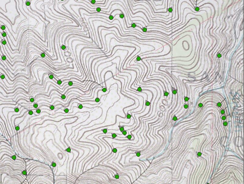
Photographed images were difficult to register due to paper stretch, folds,
and distortion. Accuracy issues are illustrated in Figure 1. Time did not permit
correction of these data for this preliminary analysis, but that will be done
in the future.
 Figure
1. The contours of the 1977 map are identical to those displayed on the USGS
quadrangle that was imported into ArcGIS. The match is excellent in the center
of the image, but duplicate lines indicate skew and stretch of the photographed
debris flow source map.
Figure
1. The contours of the 1977 map are identical to those displayed on the USGS
quadrangle that was imported into ArcGIS. The match is excellent in the center
of the image, but duplicate lines indicate skew and stretch of the photographed
debris flow source map.
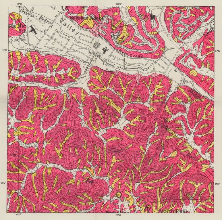
The hand-created debris flow susceptibility map has very smooth boundaries
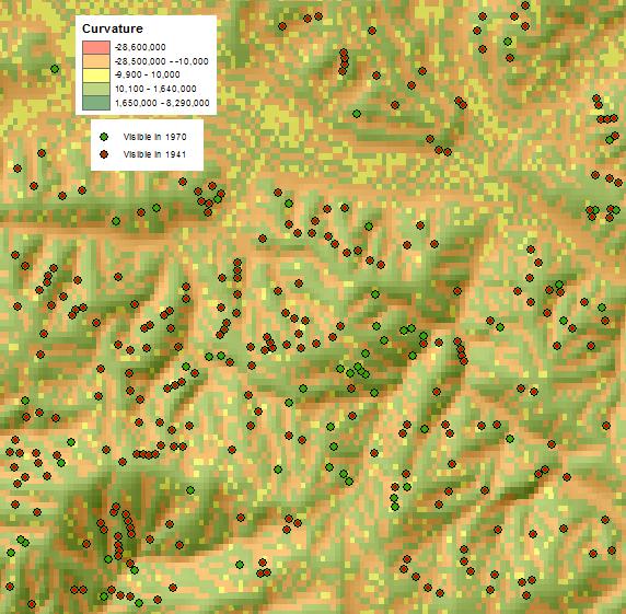
(Figure 2). In comparison, the 1 ArcSec (30-m resolution) elevation raster obtained
by USGS produced a noticeable pixilated version of a hillshade and curvature
map (Figure 3). Figure 4 shows the effect of using 1/3 ArcSec (10-m resolution)
elevation data.
 Figure
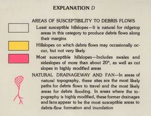
2. Hand-created debris flow susceptibility map from Smith (1988, plate 13D).
Figure
2. Hand-created debris flow susceptibility map from Smith (1988, plate 13D).
 Figure
3. Hillshade and curvature map produced using 1 ArcSec elevation data from USGS.
The 30 m resolution produced noticeable pixilation. The separation between convex
and concave slopes was purposefully narrowed in this analysis. Note that masks
for areas with slopes less than 20% or underlain by alluvium were not applied.
Figure
3. Hillshade and curvature map produced using 1 ArcSec elevation data from USGS.
The 30 m resolution produced noticeable pixilation. The separation between convex
and concave slopes was purposefully narrowed in this analysis. Note that masks
for areas with slopes less than 20% or underlain by alluvium were not applied.
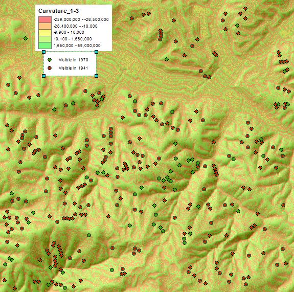 Figure
4. Hillshade and curvature map produced using 1/3 ArcSec elevation data from
USGS. The 10 m resolution reduces pixilation. As in Figure 3, the separation
between convex and concave slopes was purposefully narrowed in this analysis.
Note that masks for areas with slopes less than 20% or underlain by alluvium
were not applied.
Figure
4. Hillshade and curvature map produced using 1/3 ArcSec elevation data from
USGS. The 10 m resolution reduces pixilation. As in Figure 3, the separation
between convex and concave slopes was purposefully narrowed in this analysis.
Note that masks for areas with slopes less than 20% or underlain by alluvium
were not applied.
Analysis
The 10 m elevation data produces a noticeable improvement in the resolution
of the hillslope analysis. While there are green pixels within red swales, and
red pixels on convex ridge tops, they tend to be much smaller. Additional geoprocessing
and adjustment of the curvature break parameters might remove those artifacts.
Conclusion
Higher resolution elevation data produces a noticeable change in the detail
of the analytical output. Rather than requiring days to weeks to analyze a four
square mile area, this type of analysis takes minutes, depending on the extent
of the area and whether digitized geologic maps are already available for the
area to be analyzed.
The next steps in the investigation are to redigitize the debris flow sources,
then compare those locations with the 1/3 ArcSec curvature maps to help refine
curvature break values. Masks also need to be applied to eliminate slopes of
less than 20% and alluvial areas, as well as using ArcGIS hydrology tools to
the map stream network. Additional analysis also needs to develop a method of
automatically identifying debris flow fans. Finally, higher resolution LIDAR
data might be useful for determining whether small artifacts in the 1/3 ArcSec
elevation data are real, whether a buffering function might help smooth the
product and produce regulatory maps that are easier to apply, and whether the
1/3 ArcSec data have a resolution that is good enough to develop maps for National
Flood Insurance Program purposes.
References
- Ellen, S,D., Mark, R.K, Wieczorek, G.F., Wentworth, C.M., Ramsey, D.W.,
& May, T.E. (1997). Map showing potential debris-flow source areas in the
San Francisco Bay region, California. U.S. Geological Survey, Open-File
Report 97-745 E. Retrieved from http://pubs.usgs.gov/of/1997/of97-745/of97-745e.html
- Smith, T.C. (1977). The debris avalanche: a commonly overlooked geologic
hazard. Geological Society of America, Abstracts With Programs, 9(4),
502.
- Smith, T.C. (1988). A method for mapping susceptibility to debris flows,
with an example from San Mateo County, in S.D. Ellen and G.F. Wieczorek
[eds.], Landslides, floods, and marine effects of the storm of January 3-5,
1982, in the San Francisco Bay region, California. U.S. Geological Survey,
Professional Paper 1434, Contribution No. 10, p. 185-194, Plate 13.
The text of the entire Professional Paper is available online at http://pubs.usgs.gov/pp/1988/1434/pp1434.pdf
; plates are available at http://ngmdb.usgs.gov/Prodesc/proddesc_4882.htm