TitleCalifornia Native Tree Species Distribution MappingAcquiring Spatial Information from Scanned Documents | |||||||||||||||||||||||||||||||||||||||||||||||||||||||||||||||||||||||||||||||||
|
Author
Konrad D. Pehl American River College Geography 350: Data Acquisition in GIS; Fall 2015 Contact Information: w1576625@apps.losrios.edu | |||||||||||||||||||||||||||||||||||||||||||||||||||||||||||||||||||||||||||||||||
|
Abstract Maps from the Griffin and Critchfield 1972 publication "The Distribution of Forest Trees in California," were obtained in a scanned PDF format. Maps were imported into ArcMap 10.3 and georeferenced. The maps were compared to other available printed and digital formats to assess the level of usefulness of digitizing these maps for resource inventory and research. Maps were found to be useful to delineate species location to the county and USGS 7.5 minute quadrangle level. Maps were not suitable for delineation to the public land survey section level (square mile). | |||||||||||||||||||||||||||||||||||||||||||||||||||||||||||||||||||||||||||||||||
|
Introduction The topographic and climatic diversity of California provides for a varied assortment of tree species. Because of the important ecological and economic of roles of trees, there have been various tree species mapping efforts in California. From 1928 to 1940 the Vegetation Type Map (VTM) survey of California worked on this effort. In 1947 the State Cooperative Soil-Vegetation (SV) survey replaced the VTM survey as the major vegetation mapping project in California. These efforts gathered a substantial amount of information. Some of this information was published in scattered sources, often in the form of small-scale distribution maps printed on paper. In 1972 Griffin and Critchfield published, The Distribution of Forest Trees in California. They described their effort as a "preliminary atlas." It is the best effort that I have found. Their atlas contained 84 maps of individual tree species. The base map contains county borders and is at an estimated scale of 1:5,500,000 (1 inch equals approximately 86 miles). Subsequent publications have borrowed from this effort, usually printing in a smaller scale and lower resolution. An effort to revisit the work of Griffin and Critchfield (and the work of their cartographer Audrey E. Kursinski) could have value to future researchers in the subjects of dendrology, ecology, wildlife habitat, and climate change. | |||||||||||||||||||||||||||||||||||||||||||||||||||||||||||||||||||||||||||||||||
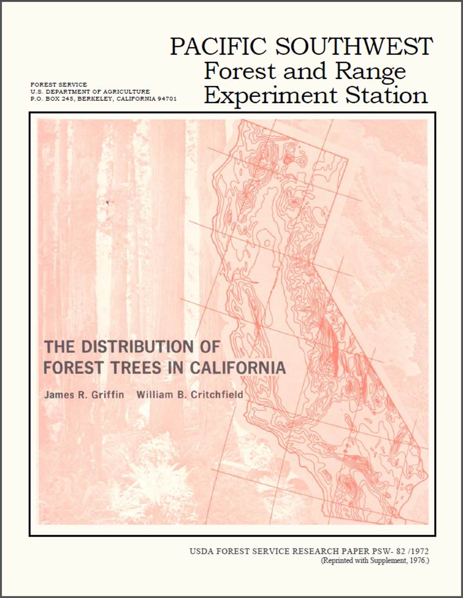
Figure 1. | Cover to USDA Forest Service Research Paper PSW-82. Publication includes 84 tree species distribution maps based on a compilation of vegetation survey work from 1928 to 1972.
| Background Internet searches for GIS data on California native tree species distribution resulted in only one digital source with statewide coverage. The source was a USGS web page (http://esp.cr.usgs.gov/data/little/). The web page contains a list of tree species with shapefiles and pdf files of maps. The maps all share the same base map of North America with U.S. States borders. They are scaled to fit an 8.5 by 11 inch page. Most of the data was attributed to being digitized from the Atlas of United States Trees Volumes 1-5, by E.L. Little (1971-78). The Atlas of United States Trees contains excellent maps. The scale of these maps vary from covering the entire western United States in one 9.25 by 11.75 inch page (approx. scale 1:10,000,000) to covering all of North America on the same sized page (approx. scale 1:32,000,000). The continental scale of these maps limits the utility of these maps. Fortunately Griffin and Critchfield published a similar series of maps at a scale that covered the state of California in one 8.5 by 11 inch page (approx. scale 1:5,500,000). I have not been able to find GIS versions of these maps. I was able to find the Griffin and Critchfield maps scanned in PDF format. I wanted to determine if these maps were of sufficient quality to be useful if digitized.
| 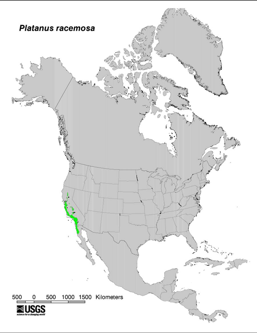
Figure 2. | Species distribution map for Platanus racemosa (California sycamore) from the U.S. Geological Survey. Scanned and digitized in 1999 for use in vegetation-climate modeling studies from Little, E.L., Jr., 1976, Atlas of United States trees, volume 3, minor Western hardwoods: U.S. Department of Agriculture Miscellaneous Publication 1314.
| 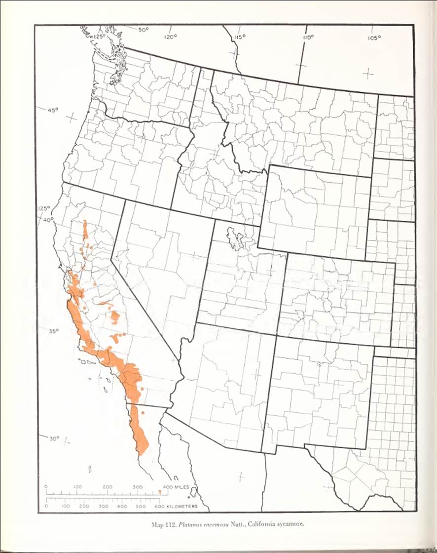
Figure 3. | Species distribution map for Platanus racemosa (California sycamore) from Little, E.L., Jr., 1976, Atlas of United States trees, volume 3, minor Western hardwoods: U.S. Department of Agriculture Miscellaneous Publication 1314.
| 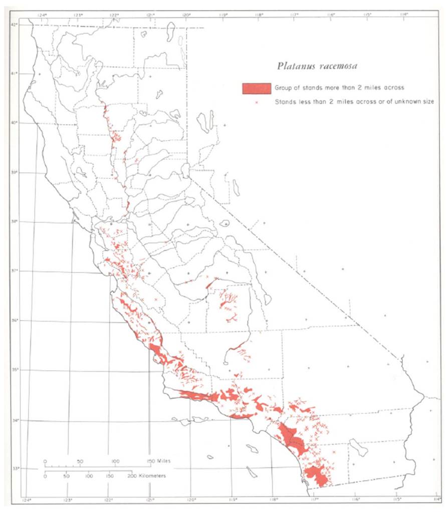
Figure 4. | Species distribution map for Platanus racemosa (California sycamore) from Griffin, James R., and William B. Critchfield 1972. The distribution of forest trees in California.
| In California, biological researchers commonly search the California Natural Diversity Database (CNDDB) for information on the occurrence of plant and animal species. This database is maintained by the California Department of Fish and Wildlife. The database is a subscription based service, with a free, web-based CNDDB Quick Viewer (https://map.dfg.ca.gov/bios/?tool=cnddbQuick). The Quick Viewer will generate a list of taxa for a given area. Search areas are designated by county or USGS 7.5 minute quadrangle area. I was interested in determining if the Griffin and Critchfield maps were of sufficient quality to add tree species data to the CNDDB. At a minimum this would require that the maps be of sufficient resolution to determine the tree species location to the county level and to the 7.5' quadrangle level.
| 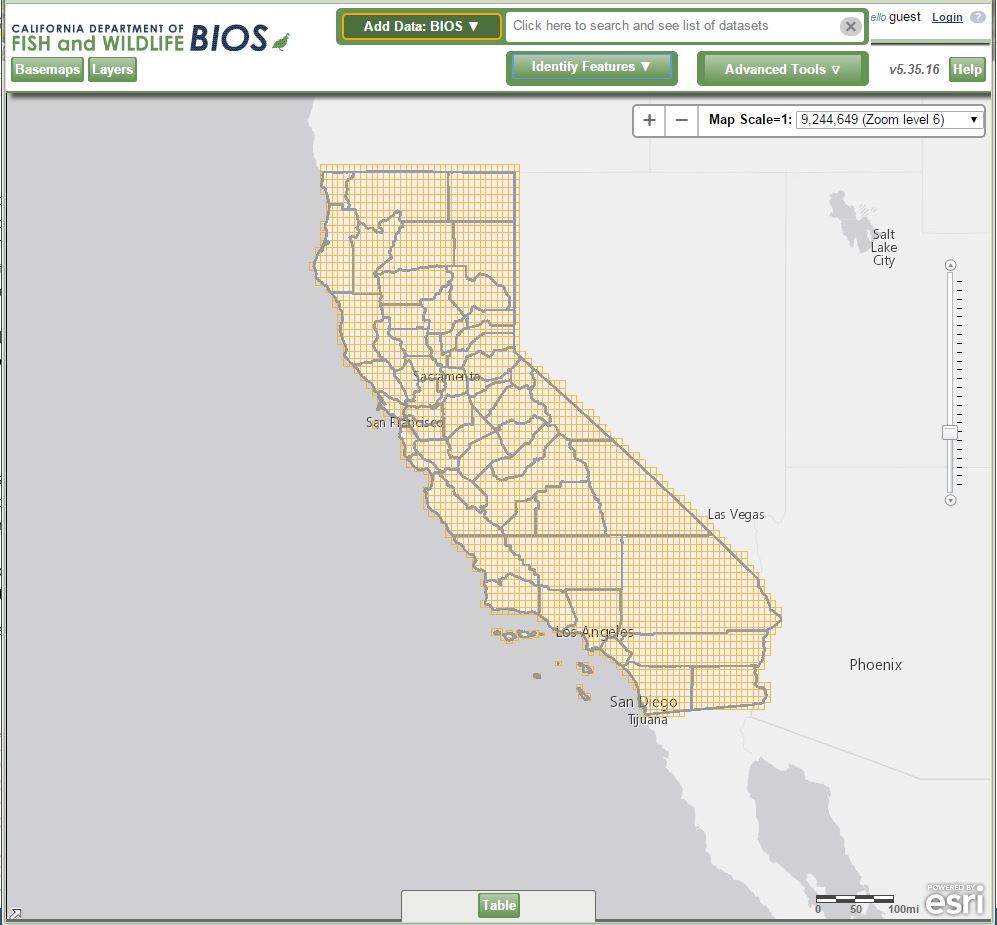
Figure 5. | Screen capture of the California Department of Fish and Wildlife's Quick Viewer for the California Natural Diversity Database. Species lists are generated by county or USGS Quadrangle. The yellow squares are USGS Quadrangles.
| Methods A PDF copy of The Distribution of Forest Trees in California was downloaded from the US Forest Service website. The scanned document was 124 pages long. The document was split into individual one page files with the Free PDF Splitter utility from freepdfsolutions.com. Selected page files with maps were brought into ArcGIS 10.3 with the PDF to TIFF tool. The image was then georeferenced by referencing the map graticule to a 1 degree grid from ArcGIS online. The georeferenced image was then evaluated by overlaying: a 1 degree graticule, a map of the counties of California, a shapefile of the outlines of USGS 7.5 minute quads, and the public land survey system section lines. The map for Platanus racemosa (California sycamore) was chosen for this example. I used this species because its distribution is wide, but many of the stands are small and are represented as point features. In addition I was able to find other map sources for its location.
| Results The map was referenced to a 1 minute grid from ArcGIS online. Total RMS error was 660 meters. This seemed reasonable for a hand draw map from a publication printed in 1976 that was later scanned in 2007. The map was visually inspected. At full page view, the 1 degree grid matched the graticule and grid ticks. At closer inspection it was obvious that with was a hand drawn map, and accuracy was limited by the width of a pen stroke. This process could have been improved if: The original prepublication master maps were located and scanned; the scanning was at a higher resolution; a reference to the original projection was found; and there was some metadata included with the 1 degree grid from ArcGIS Online.
| 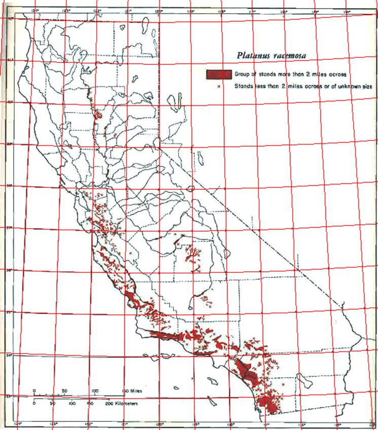
Figure 6. | Georeferenced map with overlay of 1 degree Graticule from ArcGIS Online shown in red.
| 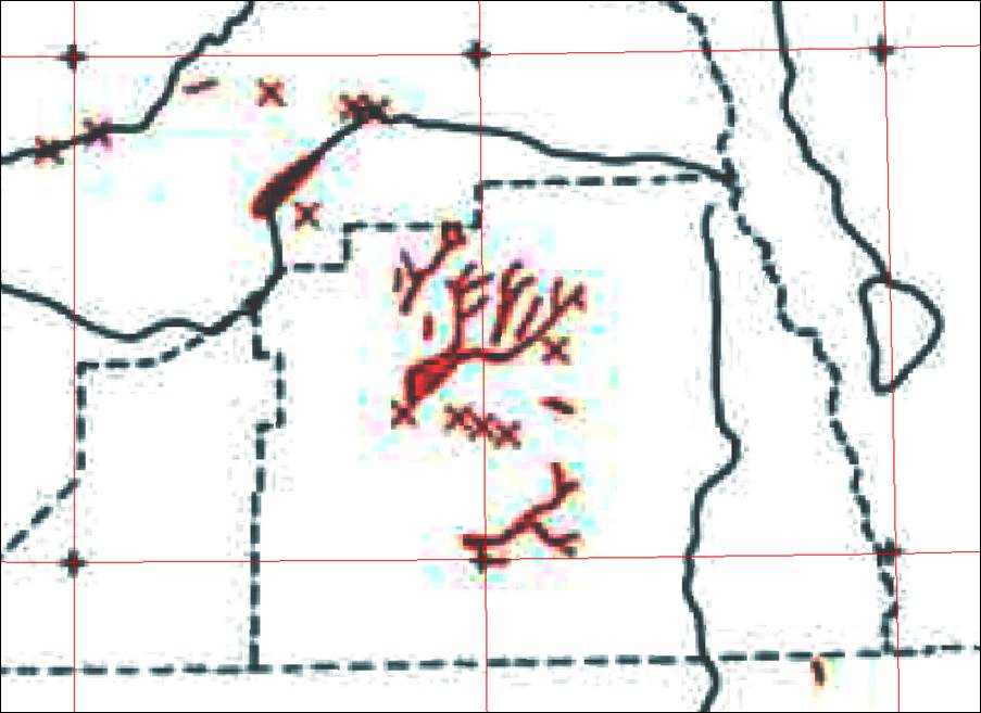
Figure 7. | Detail of Tulare County with overlay of 1 degree graticule from ArcGIS Online shown in red. Note graticule intersection with tick marks.
For a second comparison the map image was compared to an overlay of county borders.
The borders were from the California Department of Fish and Wildlife. The quality of these borders were
discussed in the metadata. Apparently the department spent considerable effort researching and sorting
through various sources of lines before adjusting and accepting this dataset. Comparison of the Griffin
and Critchfield lines with the Fish and Wildlife dataset showed variations of up to 1800 meters for relatively
straight lines, and up to 3000 meters for borders that were rivers. Much of this variation could be
attributed to the scale differences between the data sources. The Fish and Wildlife line work was from
1:24,000 maps from the USGS and U.S. Census Bureau. The Griffin and Critchfield maps used a 1:5,500,000 base map.
In some instances the maps just had the county borders in different places. |
| 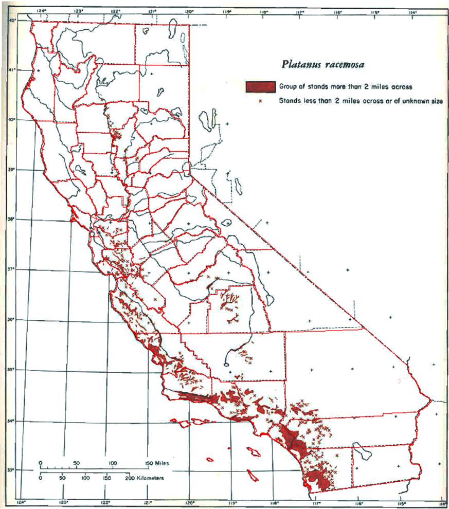
Figure 8. | Georeferenced map with overlay of county borders in red from the California Department of Fish and Wildlife.
| 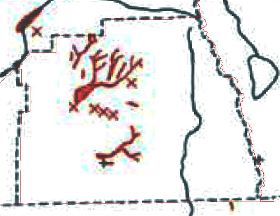
Figure 9. | Detail of Tulare County with overlay of county borders in red from the California Department of Fish and Wildlife. Note consistency / inconsistency of with dashed black border lines.
The third comparison was an examination of the mapped stands to the grid of USGS 7.5 minute quadrangles.
The mapped stands were polygons, and points for stands less than 2 miles across. At close inspection it was easy
to tell which quads the stands were contained. |
| 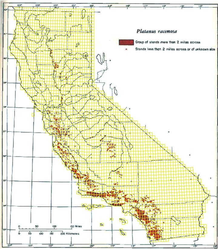
Figure 10. | Map georeferenced with overlay of USGS 7.5 minute quadrangles in yellow. Compare to Figure 5.
| 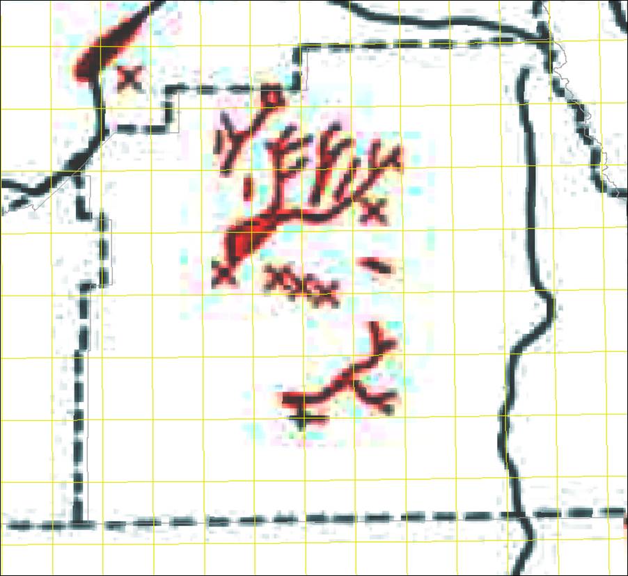
Figure 11. | Detail of Tulare County with USGS 7.5' Quadrangle overlay. Shows detail sufficient to determine species occurrence in individual quadrangles.
| 
Figure 12. | Detail of Exeter USGS 7.5 minute quadrangle in Tulare County. Shows detail sufficient to determine species occurrence in individual quadrangles.
The Public Land Survey System (PLSS) is the surveying method developed and used in the United States to plat, or divide,
real property for sale and settling. A basic unit of the PLSS is the section. The section is an area nominally one square mile
(2.6 square kilometers), containing 640 acres. Since land parcels are commonly described by the section they contain or
portions of sections they contain, I wanted to compare the map image to an overlay of sections. At page view it was obvious
that the section lines overwhelm the map. They are too dense to be resolved at the page view scale. Closer inspection also
reviewed that the map is not suitable for this level of detailed inspection. Point features of areas less than 2 miles across
are plotted as an 'X' that is 4 miles across. |
| 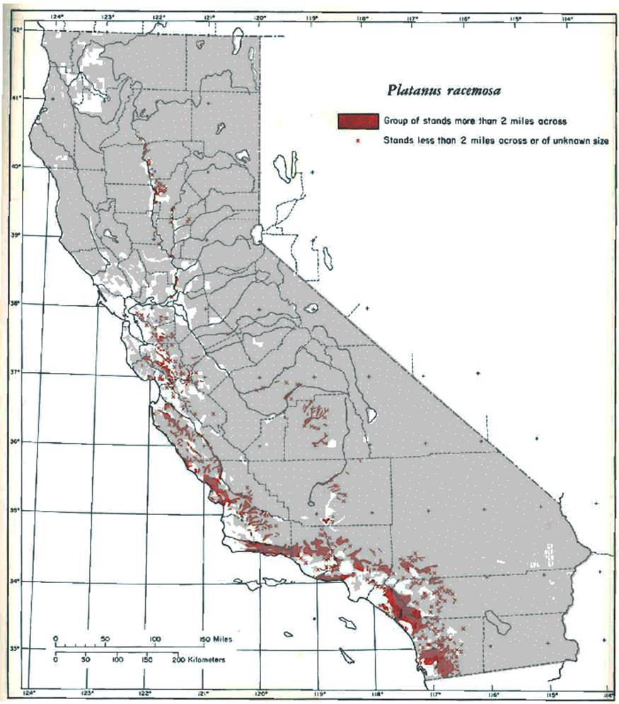
Figure 13. | Map georeferenced with Public Land Survey Section Lines Overlay in Gray. Note how detail of section lines overwhelms image at this scale.
| 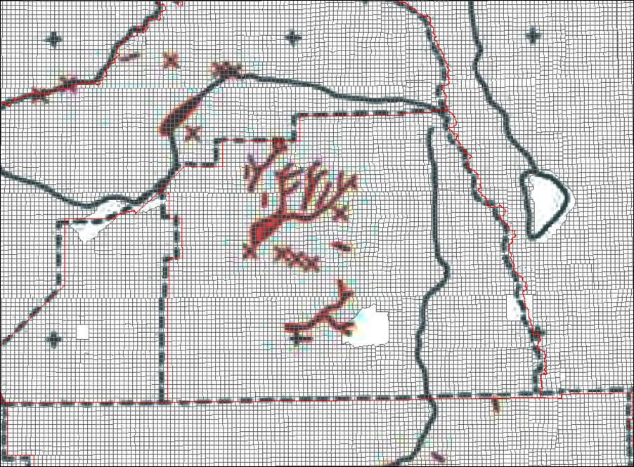
Figure 14. | Detail of Tulare County with Public Land Survey Section Lines Overlay. Note how 'X' marks are approximately 4 miles wide and are used to indicate occurrences of less than two miles wide.
| 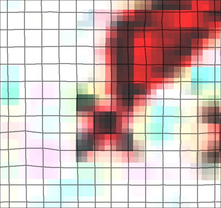
Figure 15. | Detail of Tulare County with Public Land Survey Section Lines Overlay. Note how center of 'X' and polygon edge blur into several sections.
| Analysis
The intent of this evaluation was to determine if the maps from
the Griffin and Critchfield publication were suitable for digitization and research use. The scanned documents
are of sufficient quality to georeference. The test of research use was to determine if the maps could be
used to resolve locations to the county, USGS Quad, and PLSS section. This is similar to a California Natural Diversity Database query.
Locating the occurrence to the county level was achievable, but somewhat complicated around the border which vary by map source.
Since the stand locations were plotted without reference to county border locations this is not a problem.
The comparison of stand locations to the grid of USGS 7.5 minute quadrangles begins to test the resolution of the original map.
A 7.5 minute map is printed at 1:24,000, the Griffin and Critchfield maps were printed at approximately 1:5,500,000.
The source PDF was scanned at somewhere between 200 and 250 dots per inch. Pixel size of the image in ArcMap was approximately 530 meters wide.
The 'X' marks used for small stands are approximately 5,300 meters wide (10 pixels wide). A 7.5 minute quad (north to south) is
11,865 meters wide (22 pixels wide). Generally the center of a 10 pixel wide 'X' can be assigned to the appropriate 22 pixel wide
quadrangle. This issue of resolution is somewhat reduced by the fact that researchers commonly generate species list of the quadrangles
adjacent to their area of interest in a "nine quad search." The researcher understand that much of the database information predates the age
of GPS.
The comparison of the map to the PLSS section overlay demonstrated the overextension of the original data.
The use of 1:5,500,000 scale data from a hand drawn map is inappropriate at the 1 square mile level.
| Conclusions Maps from the publication are of sufficient resolution to recover spatial information to
locate tree species to County, USGS 7.5 minute quad, but not to public land survey section.
| References Griffin, James R., and William B. Critchfield 1972. The distribution of forest trees in California. Berkeley, Calif.
Pacific SW. Forest & Range Exp. Stn. 114 p., illus. (USDA Forest Serv. Res. Paper PSW-82) (Reprinted with Supplement, 1976.) http://www.fs.fed.us/psw/publications/documents/psw_rp082/psw_rp082.pdf Kelly, Maggi, Ken-ichi Ueda and Barbara Allen-Diaz 2007. Considerations for ecological reconstruction of historic vegetation: Analysis of the spatial uncertainties in the California Vegetation Type Map dataset. Berkeley, Calif. Plant Ecology, Volume 194, Issue 1, pp 37-49. Kelly, Maggi, Barbara Allen-Diaz and Norma Kobzina 2005. Digitization of a Historic Dataset: The Wieslander California Vegetation Type Mapping Project. Berkeley, Calif. Madroño, Vol. 52, No. 3, pp. 191-201 Little, Elbert L. 1978. Important Forest Trees of the United States. Washington, D.C., United States Department of Agriculture 70 p., illus. (Agricultural Handbook 519) Little, Elbert L. 1971-1978. Atlas of United States Trees Volumes 1-5. Smith, Martyn J. and Cromley, Robert G. 2006. Coastal survey maps: from historical documents to digital databases. UCCGIA Papers and Proceedings, No. 1. Storrs, Connecticut: University of Connecticut Center for Geographic Information and Analysis. Bureau of Land Management. 2011. Cadastral PLSS Standardized Data - PLSSFirstDivision - Version 1.0. http://www.geocommunicator.gov/shapefilesall/CadNSDI/CA_PLSSCADNSDI_09192011.zip California Department of Fish and Wildlife. 2011. County Boundaries (24K). ArcGIS shapefile. Free PDF to TIFF Converter, http://freepdfsolutions.com/
| |