Title

             A Comparative Study of Drought Effects on Wildfire Levels In Northern California

Author

Shawn Stiver

Geography 350: Data Acquisition

American River College

Professor Paul Veisze

Abstract


In 2012, California entered a drought period throughout the state. A common notion is that drought also brings with it a rise in wildfire size and frequency. Lack of precipitation plays a major part in affecting the amount of fuel available for a wildfire; the lack of moisture contained in groundcover may increase the likelihood or the intensity of a wildfire. So while it is easy to assume that wildfires may be more common and larger in size during a drought, what are the actual numbers? This study used precipitation and wildfire data for the years 1980 through 2014 to attempt to find a correlation between drought and wildfire frequency and effects. This project used ArcGis 10.3 ModelBuilder to construct a process for the extraction and preparation of data pertinent to this timeframe. Analysis from this project was inconclusive, due to the simplistic nature of the model for an extremely complex relationship.

Introduction


Since 1980, California has entered two periods of extreme drought. The first period was from 1987, through 1992, and the 2nd period began in 2012 and extends through present day. 2014 was the driest period ever recorded in California history, with records extending back to 1849. This lack of precipitation has had a great number of negative effects on the state:  restricting agriculture, mandatory water rationing by the general populace, and multiple impacts on the environment. The summer of 2015 brought a number of catastrophic wildfires throughout the state, resulting in loss of life, damage to millions of acres of habitat, and the destruction of thousands of homes and structures. A common theme in the reporting of these wildfires was the effect of the current drought aggravating the ferocity and size of these disasters. While wildfires certainly do take place during non-drought years, common sense dictates that they would not be as frequent or as large as during drought years. This study is an attempt to compile data on both precipitation levels and wildfires and identify any correlation between the two phenomena.

Background


  The relationship of drought and wildfire in California is an extremely complex phenomena. There is no doubt that drought conditions contribute to conditions that are favorable for wildfires in California. Drought conditions contribute to the die-off of vegetation, adding to the amount of fuel available. Low humidity levels in the atmosphere contribute to the aggressiveness of wildfires, leading to larger losses of acreage. Previous studies of the relationship of drought and wildfire levels have considered an enormous number of factors such as climate, terrain, vegetation and meteorology. The enormous amount of data required for these studies was outside the scope of this project due to time constraints.

Methods


Precipitation Data

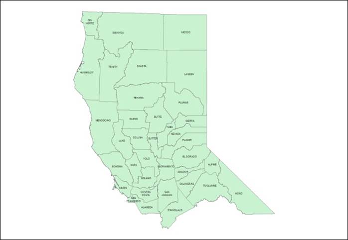
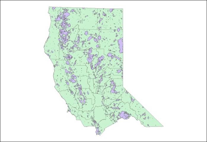
In an attempt to limit the scope of this project, the study area was limited to the northernmost counties of California (Figure 1) and restricted to the time period between the years 1980 and 2014, the last year wildfire data was available. Data used in this study was obtained from two sources. Precipitation data was downloaded from the NOAA Climate Data Online website, http://www.ncdc.noaa.gov/cdo-web/ in CSV format. Precipitation data was limited to one station per county due to restrictions of website download size restrictions and project timeframe.  Station selection was dictated primarily by the completeness of the data, many stations had considerable gaps in a 34 year timeframe, or had ceased operation at some point.


Figure 1. Northern California Study Area


The raw data downloaded presented some challenges in its raw format. Annual summaries of precipitation were presented as totals of each month. For 24 years of precipitation data over 36 counties, the raw data was composed of 13, 833 lines of data. Values for rain and snow values were lacking decimal points, and date values were presented in aggregated form for month and year. For example, January, 1980 was presented as 198001.


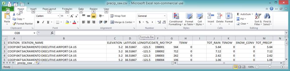
Excel was used as the primary step for processing the data into useable form. Decimal points were calculated for precipitation values by multiplying the values by the appropriate multiplier (564 x .01 = 5.64”). Snow values were converted to inches in the same fashion then converted to equivalent rain values using an average of ten inches of snow equals one inch of rain (National Weather Service). Rain and snow values were then added together to determine total precipitation for that station. (Figure 2) Total precipitation values of zero were then removed as they would play no part in calculating values and could be problematic in averaging values. The data was then saved in CSV format.


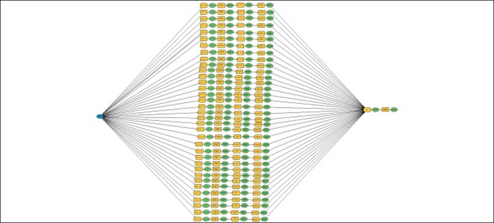
Figure 2. Precipitation Pre-Processing


The next step in processing the data consisted of importing the data into ESRI ArcMap 10.3. The processed CSV file was brought into ArcMap, and a Project X/Y Data operation was performed, using a NAD 1983 Albers projection in order to match with the wildfire data addressed later in this study.  This was then exported to a permanent feature class in ArcMap for further processing.


Several additional operations were required to process the data into a useable form for this study, and performing the steps manually for each of the 34 years of data would have been prohibitively time extensive, especially if experimentation with different values were to be attempted. To address this, a model was utilized for extracting and processing the raw data into useable form. (Figure 3)


Figure 3. Precipitation Data Model


Each row represents a year included in the study. Several steps were required to process the raw data into useable form. (Figure 4)


Figure 4. Precipitation Processing


The first step in processing was to extract the data by year. For this a Select By Attribute operation was used. Since the year was in a format including the month,  a “LIKE” expression was used to isolate the value required and save it to individual tables containing data only for that year (DATE LIKE '%1981%'). This table was then summarized by the location name to determine the sum total and mean each location that year. An additional field was then added to the table and the Calculate Field operation was used to add a “YEAR” field to the table to simplify downstream operations on the data. (Figure 5) Frequency values do not add up to 12 (months) due to in some cases incomplete records for the station, or the removal of “zero” values performed in pre-processing.


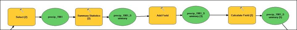
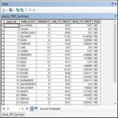
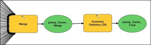
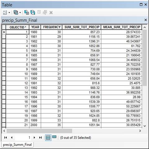
Figure 5. Summary Table by County and Year


The last step of the process was then to merge the individual summaries into one table using the Merge and Summary operations (Figure 6) into a final table output. (Figure 7)


Figure 6. Final Merge and Summary Operations.


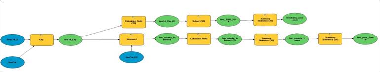
Figure 7. Final Output Table


Fire Data

The wildfire data used in this project was obtained from the Cal Fire FRAP (Fire and Resource Assessment Program) at http://frap.fire.ca.gov/.  The data used for this study was aggregated from a number of governmental agencies, and consists of a wealth of data regarding wildfires in California dating back to 1878. The data was downloaded in shapefile format and did not require the level of preprocessing required with the precipitation data.


As with the precipitation data, a model was constructed in ESRI ModelBuilder to process the data for use in this study (Figure 8)


Figure 8. Wildfire Data Model


The first step in processing the data was to clip the shapefile to the area of the study using the county shapefile to limit the extent of the data. (Figure 9)


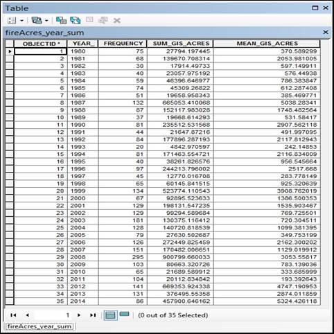
Figure 9. Clipped Fire Shapefile


After clipping, the model splits into two paths. The upper path was used to calculate total values for the study area. The lower path was used to generate data relating to individual counties, and is not discussed in the study.  Following the upper path, the GIS_ACRES field was recalculated to update the values of the features affected by the clip. As an interesting note, recalculating an area in ModelBuilder is not as simple as right clicking on the field and click “Recalculate Geometry” as would normally be done on an individual attribute table. It required use of the Calculate Field tool, using a Python expression !shape.area@acres! to update the values.  A Select operation was then performed that selected data pertinent to the study, removing features occuring prior to 1980, and intentionally set (controlled burns) from the dataset.  A Summary Statistics operation was then performed, resulting in a final table that showed sum totals and mean values for acreage burned by year (Figure 10).


Figure 10. Final Fire Summary Table

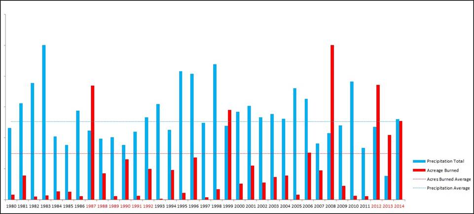
Results

After the final summaries for precipitation and wildfires were generated, they were exported into XLS format, and Microsoft Excel used to generate graphs for presentation. All values were normalized as a percentage in order to allow side by side comparison. Drought years are highlighted in red at the bottom of the graph.  The final outputs are displayed in Figure 11.


.

Figure 11. Final Output

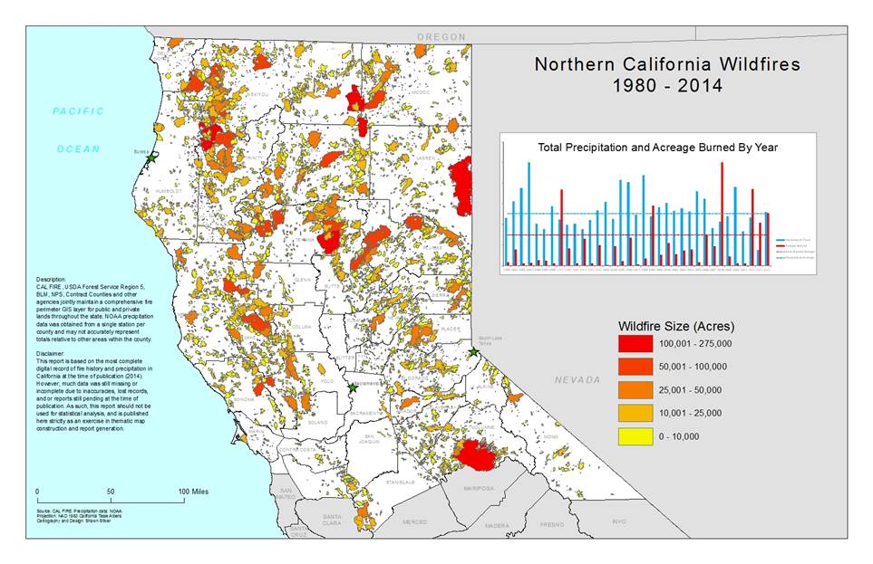
Processed Images/Maps


Analysis


Looking at the resulting graph above, there does not appear to be much correlation between the amount of precipitation and the resulting amount of acreage burned. This outcome was not unexpected, as this study consisted of a very simplistic model of an extremely complex relationship. A great number of factors were not considered in this model. First and foremost, precipitation levels were only considered from one station per county. Multiple stations in each county should have been analyzed and averaged in order to achieve a more accurate assessment of precipitation totals. Other factors in the wildfire side of the data should have been considered and weighted as well, such as fire hazard zoning, resources available, and terrain.  Unfortunately, the sheer amount of data required for such an analysis would have required months of preparation, and therefore impossible in the timeframe available for this project. However, this model can be considered a bare bones proof of concept for data processing of this subject and can be modified as time and resources allow in order to achieve a more accurate representation.

Conclusions


  Drawing direct correlations between precipitation and acreage destroyed by wildfire over a large scale would be a monumental undertaking. The variables of precipitation amounts, climatology and habitat vary wildly throughout the state, and averages of one county may not be related or have any relationship with another. The high rainfall and foliage in northern counties is just too different from the environment of southern counties to be able to draw a direct relationship between the two. This study may be effective on a smaller scale, using smaller zones within the study area in order to achieve more accurate conclusions of the relationship of drought conditions and wildfire frequency and effect.

References


Swigert, Peter. "Fire and Drought in California" 2014.05.14
http://people.ischool.berkeley.edu/~peter.swigert/fire_and_drought/  Last accessed 2015.12.10


Additional Links

NOAA Climate Data Online || Cal Fire FRAP