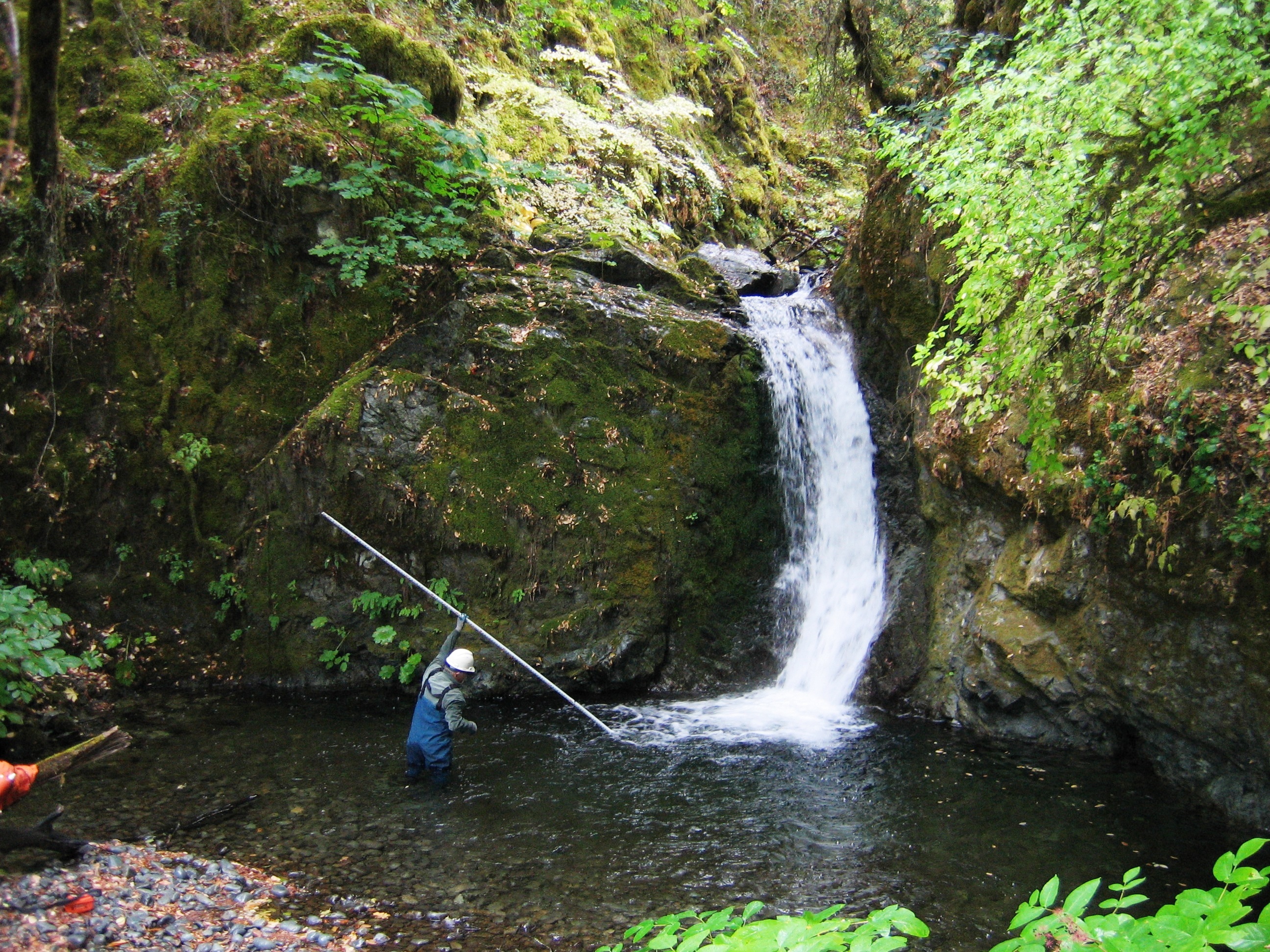
Multiple agencies and watershed groups have been working towards identifying and removing barriers to salmonids in California since the 1990's to aid in the recovery of these populations. In 1991, the California Department of Fish and Game (now Fish and Wildlife) wrote the first version of a manual for the restoration of salmonid habitat. The manual recommends completing or using existing stream inventories to identify natural limits to anadromy (i.e., waterfalls, etc.) and the suitability of habitat for salmonids downstream of these limits. Stream inventory surveys are extensive on the ground surveys that have not been completed for every stream in California nor have they been evenly distributed throughout the state. Agencies and their funding programs use the information when choosing which fish passage projects to support and fund by selecting those that will result in the most habitat gain. For streams lacking stream inventories and in lieu of completing them, the manual provides another option for estimating potential available habitat for salmonids. This option includes identifying potential natural gradient limits to anadromy where a sustained slope exceeds 8 to 10% over a distance of 1,000 feet determined from a 7.5-minute quadrangle topographic map (Flosi, 2010). Several fish passage assessments use this approach to determine natural limit to anadromy; however, other assessments have estimated limits using digital elevation models (DEMs) in streams that lacked stream inventories. This includes surveys conducted by HDR Engineering, which have done extensive surveys in California’s central valley and its coastal watersheds.

I am interested in understanding the accuracy of estimated limits to anadromy and the methods used. I will calculate gradient limits using topographic and DEM methods, and compare the results to the known limits of anadromy. I anticipate some percent error in the estimated limits capturing actual limits due to the difficulty in capturing sheer drops in gradient (e.g., steep waterfalls versus cascading falls).

Figure 1. 14-foot Waterfall on Canadian Creek, Tributary to the Trinity River in California.

Although Stoecker Ecological's assessment of Santa Barbara County used the Manual’s method to estimate limits to anadromy, where access to the stream was not possible, the assessment calculated gradient of each stream reach using the U.S. Geological Survey’s 30-meter DEM. Stoecker used the elevation at the downstream and upstream ends of each stream reach to calculate the slope of each reach using the rise (elevation/height) over run (distance/quantity of the reach) multiplied by 100. Of the 231 habitat reaches, roughly 3.5% were of reaches that were smaller than 100 meters. Stoecker developed a 1:24,000 scale stream dataset to use for the stream reaches which primarily used streams created by Santa Barbara County which were digitized from USGS 7.5 minute quadrangles. Stoecker took several dozen-stream gradient measurements in the field and compared them to the GIS-derived gradients, and overall, the GIS-derived stream gradient accurately characterized the gradient of the stream with a few exceptions. Stoecker believed these exceptions were caused by the spatial resolution of the DEM (30-meter) where elevations of nearby features (hills and cliffs adjacent to streams) assigned to the downstream and upstream ends of stream reaches (Stoecker, 2002).

HDR Engineering is another consulting firm that has completed extensive fish passage assessments in California and generally for the California Department of Transportation assessing fish passage at state highway crossings. Beginning in 2014, HDR began estimating limits to anadromy where a sustained slope of 12% or greater extends over a distance of 100 meters. HDR estimated potential habitat above highway crossings by quantifying the length of streams from these crossings to the upstream limits they estimated. HDR cited a memorandum written by R2 Consultants as the source of this methodology (HDR Egineering, 2016).

R2 Consultants conducted several literature reviews prior to committing to the method HDR generally utilized (with the exception of the resolution of the input data), which included reviews of a NOAA memorandum and a USFS presentation comparing methods for estimating stream channel gradients using GIS. It appears from this literature review, 10-meter DEMs were recommended as opposed to the 30-meter DEMs that HDR Engineering utilized to estimate limits in their assessments (R2 Resource Consultants, 2007).

Per a power point presentation by the U.S. Forest Service, which R2 consultants cited, a slope measured over a distance of 100 meters or greater is most appropriate when using a 10 meter resolution DEM nd has an average error of roughly 0.68% points (add citation – USFS presentation). USFS computed slopes using 10-meter DEM and 1:24k contours (which is the scale of the contours on USGS 7.5 minute quadrangle topographic map) and compared the results of each method to one another. The slopes calculated from each method were similar but diverged in higher gradient areas where the slopes roughly exceeded 14% which is why the DEM is preferred in high gradient areas over other methods. In addition, USFS recommended using 10-meter DEM data for elevation (rise) and high-resolution NHD to establish the distance (run) when calculating slope because NHD more appropriately represents streams and their length compared to DEM generated streams. Many of the streams in the high-resolution NHD comes from digitizing the streams in 7.5 minute quadrangle topographic maps. Per the data presented by USFS, it appears that 100 meters is the smallest distance at which gradient can be accurately estimated; however, accuracy in elevation increases as the distance increases above 100 meters. USFS conducted this analysis in Idaho (Nagel, 2006).

Per the NOAA’s technical memo, it was their general impression that using DEMs with a 10-meter resolution to identify major natural barriers to anadromy identified most known natural barriers to fish passage but failed to pick up barriers smaller than 10 meters. This impression was made after looking at the results for the Mad River watershed; however, no quantitative analysis was conducted to conclude this (Agrawal, 2005).

It appears from the research summarized above, contour lines on topographic maps and DEMs with a spatial resolution greater than 30 meter (i.e., 10 meter) are best at estimating slopes and the accepted slope used as the limit of anadromy varies from 8 to 12%. A 12% slope is determined to be the limit to anadromy in Northern California per NOAA's technical memo and is the accepted cuttoff by R2 Consultants and HDR Engineering; whereas, CDFW's restoration manual recommends using a 8-10% slope throughout the state of California.

I will use the methods discussed above to compare with the known limits to anadromy.

Figure 2. Study Area (Watersheds) and Sample of Known Natural Limits to Anadromy.

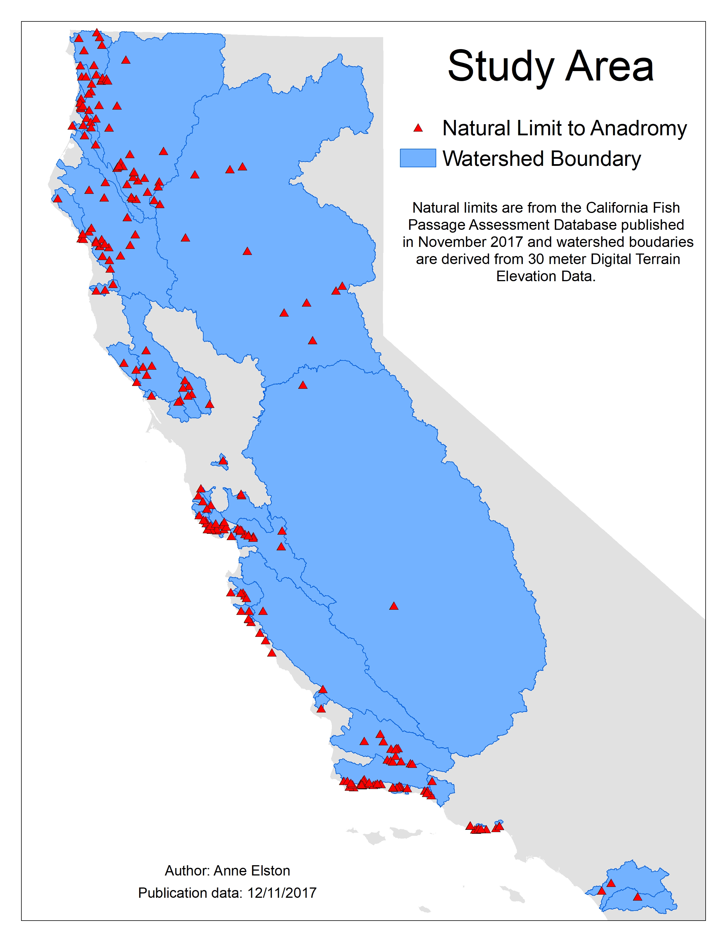
Step 1. Select, review, and create a random sample of natural barriers to anadromous fish passage to compare to estimated limits.

The feature class from the California Anadromous Fish Passage Assessment Database (PAD) published in November 2017 was downloaded from CDFW’s ftp site. This dataset was used to select all natural limits to anadromy using field surveys and professional judgement as the protocol used as specified in a definition query in ArcMap. PAD records are snapped to USGS's high-resolution Natural Hydrography Dataset which is digitized at a 1:24K scale. There is not an established protocol used to determine natural limits to anadromy in California; therefore, professional judgement is usually used in the field and recorded as either field survey or professional judgement in the protocol field. PAD records are point features and each point represents the location of a natural or man-made feature or the downstream end of these features if they are linear (in the case of gradient barriers extending over a certain distance).

I manage the PAD and I am aware of its inaccuracies due to data entry errors. Therefore, each record in the attribute table was reviewed to ensure accuracy of the records. If the text in the notes or site name fields noted that the limits were estimated using GIS or topographic maps, or there was ambiquity as to whether the natural feature may be a limit to anadromy (i.e., might or may be a limit to anadromy, barrier at most flows and stronger swimmers like steelhead can migrate upstream), then these records were selectively removed in the definition query. This subset is a more accurate dataset.

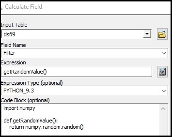
A new field was created and the field caculator was used to calculate random numbers between 0 to 1 using python code (refer to Figure 3). Using the 'Select by Attributes' tool in ArcMap, selected records where the number was less than 0.4 and exported into a new dataset to be used to compare the estimated limits of anadromy to. The export had a good sample of records geographically distributed throughout the state. This dataset was used to compare with estimated limits and it has 227 records.

Topographic maps (geotiffs), and 10 and 30-meter DEMs were obtained from the California Department of Fish and Wildlife's internal GIS repository, although these datasets orginated from the U.S. Geological Survey and are publically available online. The 30-meter DEM was already mosaiced which covered the entire state of California. A new mosaic raster was created out of individual DEMs using ArcGIS's 'Mosaic to New Raster' tool.

The stream layer referred to as California streams is maintained and published by CDFW. I obtained it online from CDFW's ftp site. The stream layer is at the 1:24, 000 scale and is similar to the high-resolution National Hydrography Dataset produced by NHD; however, the California streams feature class represents that most up-to-date hydrography for the State of California. Changes to the California streams feature class is sent to USGS for updating the high-resolution NHD.

Step 3. Create estimated limits using a 12% slope sustained (but really averaged) over a distance of 100 meters (or less) in length based on a 30-meter resolution DEM (HDR Engineering's Methodology)

This step uses HDR's Engineering methodology (12% slope over 100 meters) and modifies their process slightly to obtain this. I built a model in ArcGIS's model builder to run this process.

I used the steps that HDR laid out on pages 27 to 31 of the fish passage assessment they produced for the State Highway 1 Crossings in Marin and San Mateo Counties in California. Depressions in the DEMs (sinks) were filled in, a flow direction raster was created from which a flow accumulation grid was produced. A stream layer was produced using the flow accumulation grid, it was split into segments and average slope from the DEM was applied to each stream segment using the 'Add Surface Information' tool. The end product was a DEM-derived stream layer with average slope calcuated at each segment where each segment does not exceed 100 meters in length. Since it uses average slope, I assume the slope within each segment can vary and may vary from higher or lower slopes. I expected the streams to be split at 100 meter segments not segments at 100 or less than 100 meters. This was caused by the 'Densify' tool which was used to create vertices from which the streams where splt using the 'Split Line at Vertices' tool. When using a distance as the option to create vertices, the distance will not exceed the distance choosen, which means that the distance between vertices will be 100 meters or less which meant the legnth of the lines where 100 meters or less. Please refer to the HDR assessment for more details about their process and the individual tools used. I made some slight modifications to their process which including not clipping the DEM to County boundaries since my focus area generally covered much of the state of california, I created and used pour points at the very downstream end of the watersheds where known limits of anadromy were within, and I applied a value of 1 to the z factor parameter in the 'Add Survey Information Tool' (3D Analyst) instead of 0.01 because the unit of measure in the DEMs I used was 1; whereas, the unit of measure for the DEMs used by HDR was in centimeters.

I took the DEM-derived stream layer with average slope calculated, using a definition query to find where slope was 12% or greater and then used the 'Features Vertices to Points' tool to create points at the downstream end of these segments where slope was 12% or greater. By choosing this option, the point where the slope begins to be 12 percent or greater is choosen as the estimated natural barrier which is similar to how the known limits of anadromy are drawn. Then I used the 'Near' tool to find the closest estimated limits to known limits including a distance between the two.

Step 4. Create a estimated limits using 12% slope sustained over 100 meters based on a 10-meter resolution DEM

The following tools (in order) were used to produce the output:

i. The 'Create Points on Line' tool from the Toolbox created by Ian Broad and posted online (Broad, 2017) was used and the following parameters were specified: Input Polyline: Clipped California streams; Type: Interval by Distance; Starting Location: Beggining; Use field to set value? No; Distance: 100; and Add End Points? Both.

This created points at 100 meter intervals starting at the downstream end of the streams and working upstream. The distance of the last reach was usually less than 100 meters because stream lengths are not normally a multiple of 100. Two fields were created in the new feature class - LineOID and point_value. LineOID is the unique identifier of the stream created by this tool and applied to the points, and the point_value field is the measure along that stream also created by this tool For example, LineOIDs of 2 and a point_values of 0, 100, 200, etc. would mean a point value at the very most downstream end, 100 meters upstream, 200 meters upstream, etc.

Figure 4. Results of the Create Points on Line Tool.

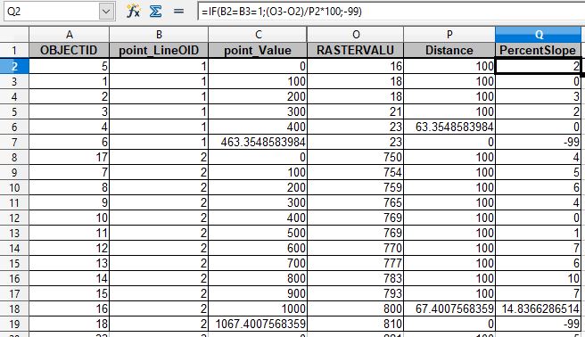
ii. The 'Extract Values to Points' tool was used to extract the elevation from DEM where it overlapped to the vector points and add them to the vector points created in step 1 above.

iii. The 'Table to Excel' tool (or Table to DBF depending on the number of records) was used to convert the attribute table of the point feature class with elevation values added to an excel file. The field for capturing the elevations was called "RasterValu".

iv. In Excel, I sorted the table by LineOID and point_Value fields which were created using the 'Create Points on Line' tool above. I added two fields, distance and percent slope, and calcuted each using formulas. Knowing that some distances are less than 100 at the end of the stream and that I am not interested in slope over distances less than 100, it was important to calculate the distance between the points. I applied the distance (e.g., the distance upstream to the next point) to the first point since I am interested in the first location where upstream the slope is greater than or equal to 12% over a distance of 100 meters. Percent slope is rise over run mutplied by 100. Therefore, I calculated the difference between the elevations at two points along the same line, deviding them by the distance, and mutiplied by 100 to obtain the percent slope. Like the calculation for the distance, the slope upstream was applied to the first downstream point.

Figure 5. Screen Shot of the Excel file and Formula used.

vi. Then in ArcMap, the excel file was joined back to its original feature class using OID as the key (join) field.

vii. Joined table to Feature class, and used a definition query selecting only where a slope was 12% or greater and where distance was 100.

Step 5. Create an estimated limits using 10% slope sustained over a 1,000 feet based on the contours on USGS 7.5 minute quadrangle topographic maps (CDFG Restoration Manual).

This process uses contour lines on topographic paper maps to calculate slope and find where slope is 10% over a distance of 1,000 feet. Contour lines in topographic maps are generally 40 feet. I tried to find a way to automate this instead at carefully looking at each contour line in the topographic map and caculate slopes. I looked at alternatives such as creating contour lines out of DEMs and using spatial files of contour lines already produced by USGS; however, these contour lines did not align with the contour lines in the topographic maps. Instead I just took a cursory look at the slopes near the known limits of anadromy.

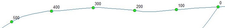
I started by zooming in on the stream with the natural limits and I looked for where the slope was about 10% over a distance of 1,000 feet and confirmed this using the measure tool. A 10% slope is about 2.5 contours with intervals of 40 feet over a distance of 1,000 feet. I created a point feature class and populated it with points at the downstream end where the slope was 10% or greater over a distance of 1,000 feet. The feature class contained fields for capturing the distance to known limits and whether the estimated limits were downstream or upstream of the known limits.

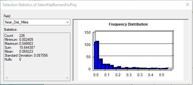
Using the steps in HDR’s assessment (e.g., average slope of 12% or greater over a distance that did not exceed 100 meters), natural limits were on average roughly within roughly 0.07 miles or 370 feet of known limits. The known historical upstream limit for Chinook runs on Kings River in the Central Valley was not picked up by this method and I suspect this is because the Central Valley is generally flat with some gentle slopes. This record (PAD ID 736824) was treated as an outlier and was not included in the analysis or graph; however, this record shows that this method may not be ideal for determining limits in low lying areas like the Central Valley and in these cases relying on knowledge of known limits would be best.

Figure 6. Graph showing the distances of estimated limits to known limits using HDR's process.

A difference of roughly 370 feet between estimated and known limits may be good enough for estimating upstream miles of potential habitat depending on the quality of that habitat. Generally, restoration efforts choose projects that open up the most amount of habitat (usually several miles) and +/- 370 feet does not account for a significant distance in potential habitat gain; however, if this 370 feet of habitat is high quality for rearing or spawning, this could persuade the prioritization and remediation of anthropogenic barriers downstream. For this reason, both the quantity and the quality of the habitat for anadromous fish should be verified by fishery biologists with knowledge of the stream.

Using the steps in Step 3 in the Methods section above (12% slope or greater sustained over 100 meters using 10-meter DEM), I found several natural barriers near known limits and on the same stream similar to the results of HDR’s process.

Although on average these estimated limits were in proximity to the known limits, the results may give a false sense of security in estimating gradient limits using these methods. Both methods (steps 2 and 3) created estimated limits lower down in the watershed and a far greater distance (several miles in a few cases) from known limits. When I compared these estimated limits to the contour lines in the topographic maps, the slope derived from the DEMs were similar in the higher elevations but differed significantly in the lower elevations. This makes me think that the slopes derived from DEMs for the streams at lower elevations are not accurate; however, this should be confirmed with fishery biologists and field verified. USFS noted that within DEMs accuracy varies and there can be errors; which is why they employed three different methods for determining slope for streams in low lying areas (valleys), streams on mid-slopes and streams on high-slopes. They used contour lines from topographic quadrangle maps for low lying areas. The estimated limits lower in the watershed could significantly reduce the estimate of stream miles upstream of anthropogenic barriers and change the priority rankings for these barriers.

Of the 20 estimated limits of anadromy I was able to digitize, the distance to the known limits varied with an average distance of roughly 1.1 miles. I ran out of time and to truly understand the accuracy of this method, I need more sample points. Due to the small sample size, this is not a fair comparison with the estimated limits derived from the DEM.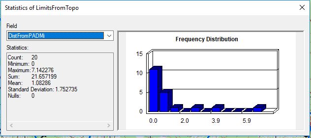

Figure 7. Graph showing the distances of estimated limits to known limits using Topographic Maps.

When I first conducted the research for the project, the methods for estimating natural limits seemed straightforward. However, when I read the reference material and each of the sources they cited, I found that the methods they choose differed from the methods identified in their source material (i.e., average slope versus slope sustained over a certain distance, different resolution of input data chosen (e.g., DEM), etc.). Initially, I expected to analyze the estimated limits determined from topographic and DEM-derived methods; however, because of the variations in the methods for deriving slope from DEMs, I had to modify and expand my project to include step 3 in the Methods section.

I had planned to conduct a quantitative analysis instead of a qualitative one, which is why I wanted a sample of known limits that contained a large number of records and were spatially distributed throughout California. The difficulty in this approach was that it was extremely time consuming to process all of the data. Some of the geoprocessing tools took days to complete. In addition, coming up with the process and figuring out which geoprocessing tools I needed to execute each method was also time consuming. Building the steps in ESRI's model builder was helpful in running the process and repeating them, as needed. When I built a model for each method, I ran each step of the model for a small geographic area and visually looked at the data produced at each intermediate step ensuring that tool used generated the result I wanted. During the running of ArcGIS's stream link tool laid out in HDR's methodology, the tool would take several days to process and either would not produce an output or process a portion of the output. I did not know the cause of this error until later, which was an ArcGIS 10.4 error. I had to install a service pack to fix the issue.

I suggest redoing this exercise beginning by focusing on a particular watershed and evaluating the estimated limits against all of the known natural limits in the PAD, instead of a sample of the known limits. I would suggest starting on a watershed on the North Coast of California and then expanding the analysis for four watersheds with each in the Bay Area, Central Coast, Central Valley and South Coast of California. It would be easier to evaluate the accuracy of the estimated limits and their methodology if you could evaluate them against all known and documented limits in a watershed. After completing this comparison, I would still suggest field-verifying the results because the natural limits of anadromy contained in the PAD are not comprehensive. The PAD was used because it is the best source of natural limits, although it may not capture all natural limits. Field-verification could focus on stream reaches where the slope was 12% or greater from the DEM calculated slope but slope was less from the contour lines in the topographic maps.

I would also suggest modifying the approach to evaluating the limit of anadromy using topographic maps. Instead of doing a cursory analysis looking at slopes from the contour lines in the topographic maps near known limits, I would suggest building an automated process starting with the following: Mosaic the topographic maps in geotiff form to a new raster, clip to a watershed or interest area, use the raster calculator to find values equal to the 5 (the value for the color assigned to contours), use the 'raster to polyline' tool to convert contours to line features, and then use intersect to intersect contour lines and streams. The process should be expanded by identifying the rest of the tools needed to calculate slope from these inputs.

I would further suggest that after running the suggested revised analysis, the three different methods for estimating slope on stream channels in valleys, mid-slope and high-slope regions that USFS discussed be evaluated for the same watersheds chosen in the North Coast, Bay Area, Central Coast, South Coast, and Central Valley.