Peregrine Falcon (Falco peregrinus) Nesting Habitat Suitability Model
for the Shasta-Trinity National Forest
2017 ©William Thein
Author
American River College, Geography 350: Data Acquisition in GIS; Fall 2017
Abstract
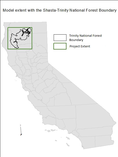
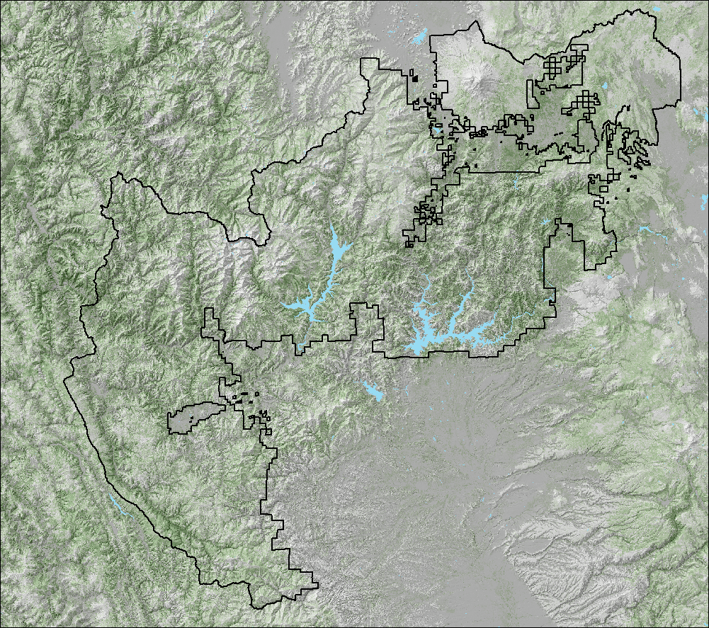
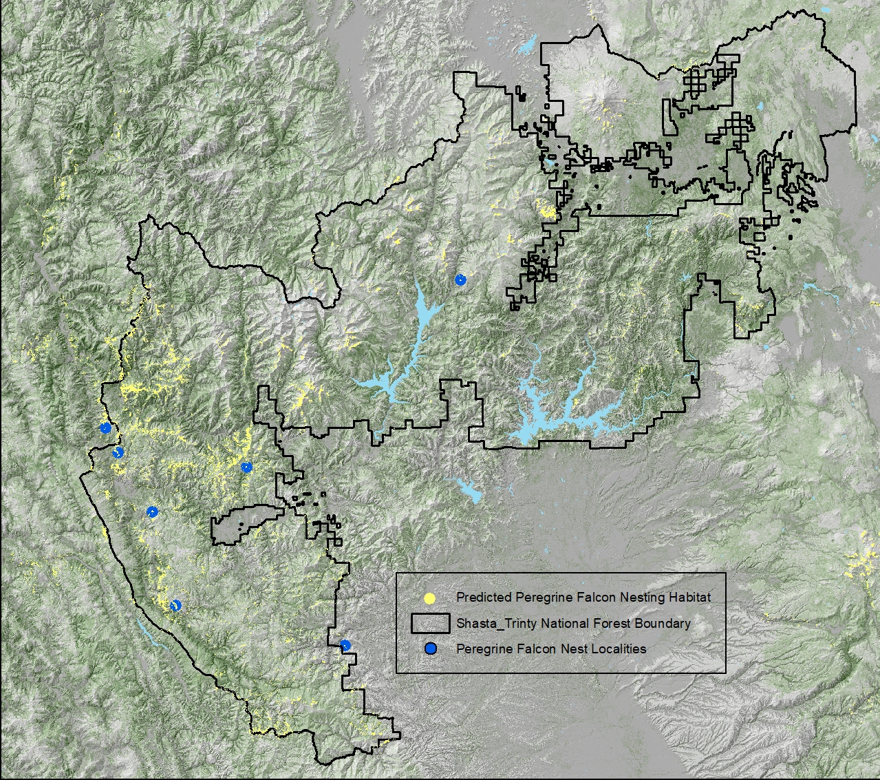
There have been little research on Northern California populations of Peregrine Falcons (Falco peregrinus) in National Forest. This project was an attempt to help focus survey efforts in the Shasta-Trinity National Forest (STNF). I was provided with Peregrine Falcon nest locality data by a raptor biologist at the Shasta-Trinity National Forest. A Maximum Entropy Model and the Maxent program to create the habitat suitability model (HSM) due to the small presence sample. Ten environmental variable as potential predictors of Peregrine Falcon nesting habitat. The variables were slope, roughness index, distance from roads, wind exposure index, distance from railroads, heat load index, distance from trails, distance from lakes, elevation, and aspect. The resulting model showed that slope, roads, and terrain heterogeneity (roughness) were the strongest indicators of Peregrine falcon nesting habitat. Unfortunately this model has low predictive value due to the elimination of many locality data points as a result of quality control standards.
Introduction
There is a fair amount of knowledge
with regard to Northern California populations of
Peregrine Falcons due to it's previous listing as
Endangered under the California Endangered Species Act
CESA) and implementation of a recovery program
(Comrack et al. 2008). There are known nesting localities recorded by the US Forest Service (USFS) within the Shasta-trinity National Forest (STNF), but to my knowledge Peregrine Falcon nesting habitat suitability modeling has not been done to determine suitable nesting sites throughout the STNF and some of the surrounding area. An off hand comment to the author about desiring a model for possible Peregrine Falcon nesting sites by a USFS raptor biologist at the STNF prompted the attempt at creating a model. A Maximum Entropy modeling approach was used to predict potential Peregrine Falcon nesting habitat using the Maxent program with 10 environmental variables.
(Comrack et al. 2008). There are known nesting localities recorded by the US Forest Service (USFS) within the Shasta-trinity National Forest (STNF), but to my knowledge Peregrine Falcon nesting habitat suitability modeling has not been done to determine suitable nesting sites throughout the STNF and some of the surrounding area. An off hand comment to the author about desiring a model for possible Peregrine Falcon nesting sites by a USFS raptor biologist at the STNF prompted the attempt at creating a model. A Maximum Entropy modeling approach was used to predict potential Peregrine Falcon nesting habitat using the Maxent program with 10 environmental variables.
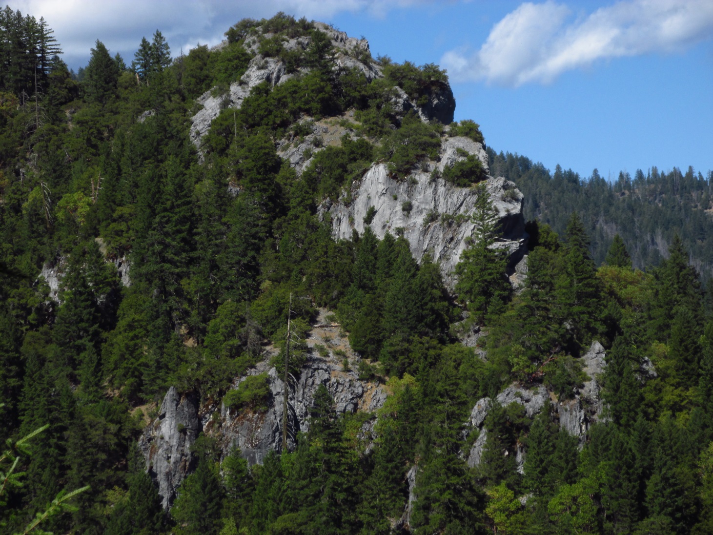
Background
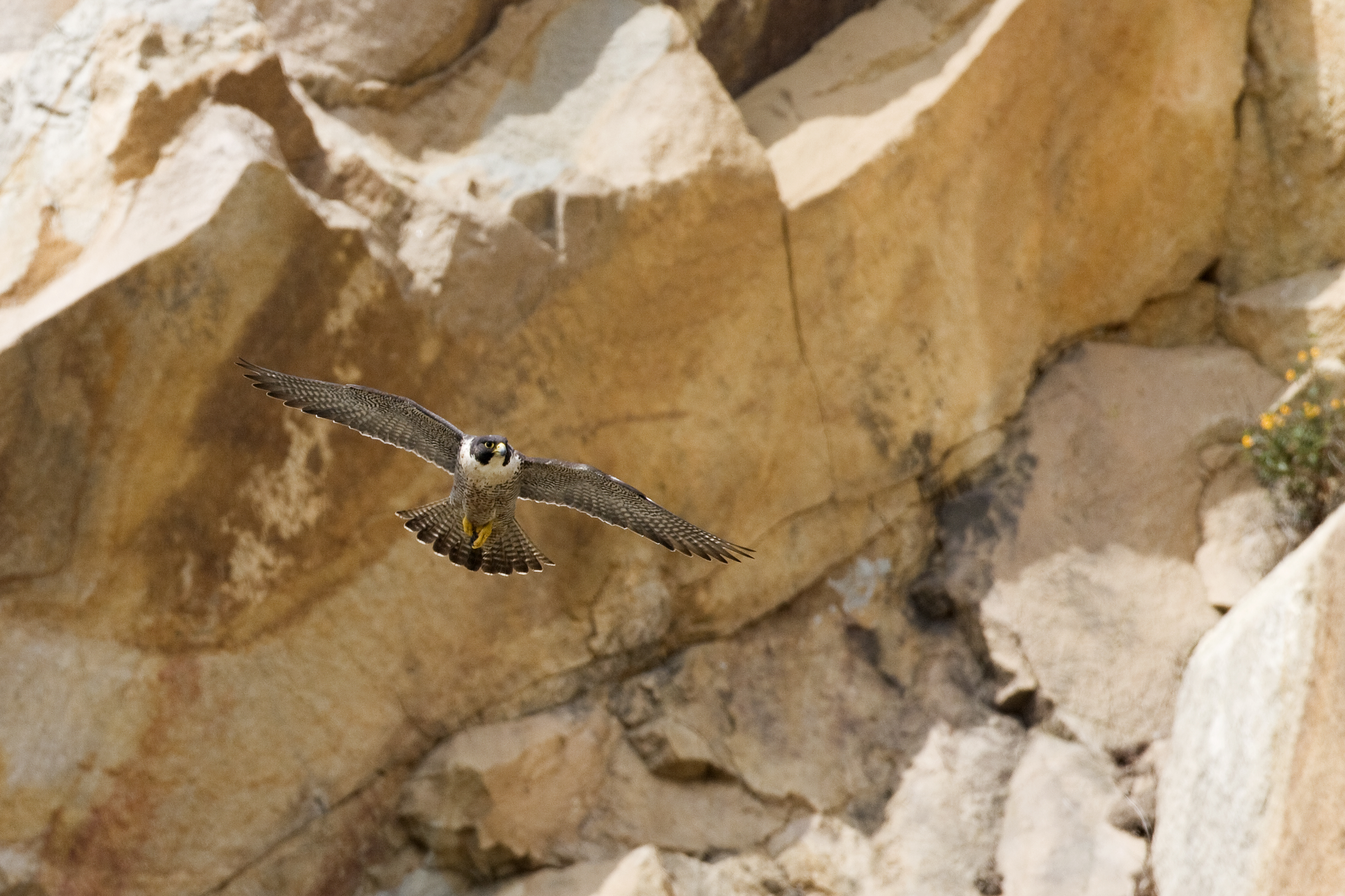
Kevin Cole from Pacific Coast, USA (https://commons.wikimedia.org/wiki/File:Peregrine_Falcon_in_flight.jpg), „Peregrine Falcon in flight“, https://creativecommons.org/licenses/by/2.0/legalcode
Methods
With the Peregrine Falcon nesting site
localities provided by William Thein of the United
States Forest Service (USFS) I began conducting
quality control checks on locality points using google
earth and the photos provided of the nesting sites
where provided. After throwing out points due to
quality control issues there were 7 nesting site
localities left. Due to the low presence sample size a
Maximum Entropy Model was used to predict possible
Peregrine Falcon nesting site habitat (Hernandez et.
al 2006).
Ten environmental variables were
selected for this model using various Geographic
Information System (GIS) programs such as ArcGIS
10.5.1, and free Open
Source programs such as SAGA
6.0.0 and
Maxent 3.4.1 (Phillips
et. al. 2017 , Conrad et.al. 2015). Aspect was
included because it may influence heat accumulation at
the nest site and possibly wind protection, the raster
was developed in ArcGIS using the Aspect (Spatial
Analyst)tool. Slope was an included as a variable due
to it's association with cliff faces, this raster was
developed in ArcGIS using the Slope (Spatial Analyst)
tool. A wind exposure index (exposure) was included as
a variable because the nesting site may need to be
sheltered from the wind, the SAGA GIS tool Wind
Exposition Index was used to create this raster Conrad
et. al. 2015). A 5m NextMap DEM was provided by Paul
Veisze for use in the class Data Acquisition (Geog
350) at American River College for these class
projects. The DEM was used as an elevation
variable in the model. Heatload was including as a
variable because it has been suggested that day time
temperatures at the nesting site may influence their
location (Barnes
2011). A heat load index was calculated with
ArcGIS using a 3rd
party ArcGIS toolbox (Evans et. al. 2014).
Distance from roads (roads) raster was created using
the ArcGIS Euclidean Distance(Spatial Analyst) tool).
Distance from trails (trails) was created using the
ArcGIS Euclidean Distance (Spatial Analyst) tool).
Distance from railroads (rxr) was created using the
ArcGIS Euclidean Distance tool. This layer was under
went manual quality control comparison using Google
Earth imagery for removal of abandoned railroads.
Because of the association with permanent bodies of
water a lakes layer (lakes) was created using the
ArcGIS Euclidean Distance (Spatial Analyst) tool. Two
different lakes layers were compared and the missing
lakes were added to a layer with the ArcGIS union
tool. A roughness Index (rough) was calculated to help
identify cliff face areas that are suitable nesting
habitat (Evans et. al. 2014). Slope is not always
indicative of a cliff and a roughness index would
possibly aid in the assessment of where cliff faces
are. A 3rd
party ArcGIS toolbox was used to create this
layer.
A nDVI/ nDSM layer was going to be used as a measure of openess/canopy height, but the values appeared wrong. I double checked and used the process nDSM = DSM - DTM using a raster calculator. The resulting nDSM again had negative values which in an ideal situation should never happen. Some error is expected possibly up to a 9m error due to differences is where the laser hits the crown and slope (Duan, Z. et. al. 2015). The negatives on a histogram were distributed well beyond
the 9m point with a minimum value of -130m. The negatives made up 12% of the entire nDSM. When plotted the negatives strangely plotted on some of the high elevation areas such as Mount Shasta essentially visually making it a caldera. Later
I did take the negatives and make them positive with the raster calculator using CON(rasterX < 0, rasterX * -1, rasterX). The resulting pattern did seem to match expectation, but still considered too dubious for use in the model. However the resulting layer was suitable for visualizations of the area. This variable was thrown out and will eventually be included once a replacement is found.
In order to create a model I chose the maximum entropy model approach due to the very small sample size and presence only data points (Hernandez et. al 2006). To create this model I used the Maxent program (Phillips S.J. 2017). Maxent has several constraints on data input that required significant storage and processing time. Some the requirements for data input are all layers must have the same extent, have the same projection, and have the same cell size. All layers must be in one of the following file formats .asc, .gri, .mxe. Locality points need to be in a carefully formatted according to a specific format and saved as a comma delimited.csv file. The created raster layers were clipped using USFS boundary polygon for the Shasta-Trinity National Forest with an added 10km buffer. The ArcGIS clip (data management) tool for rasters was used with the "maintain extent" option. In ArcGIS the resample (data management) was set to a larger 5x5 cell size to ensure a match among all layers. Rasters were then converted with ArcGIS "Raster to Ascii" tool to the .asc file type. When dealing with large files in ArcGIS and doing conversions save the output in the same folder as your source/input. I found if I did not do this ArcGIS wouldn't process the layer and give some sort of coding error. In some cases this did not work and recalculating the statics for the layer would fix the issue. After hours of processing I was met with a "java heap error" because Maxent ran out of memory because MS Windows 10 can only allocate 1.3G of RAM of continuous RAM to the program under java. The work around was to run the program under Linux which does not have this limitation and in the script file (.sh) set the memory allocation to near your max system memory. If you run into this error look to see if there is a "maxentcache" folder with your layer files converted to .mxe if so just use those as your layer files they are smaller and easier on memory usage.
Results
| Variable | Percent contribution | Permutation importance |
|---|---|---|
| slope | 34.3 | 42.1 |
| rough | 31.3 | 0 |
| roads | 21.2 | 55.2 |
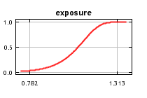
| exposure | 6.4 | 0.1 |
| rxr | 2.7 | 2.4 |
| heatld | 2.1 | 0.1 |
| trails | 2 | 0 |
| lakes | 0 | 0 |
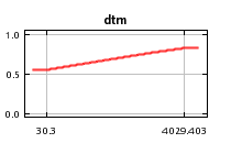
| dtm | 0 | 0 |
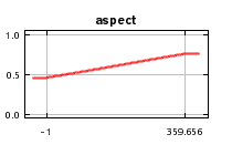
| aspect | 0 | 0 |
| Variable | Fitted-lambdas | Minimum | Maximum |
| Aspect | 0.0 | -1.0 | 359.6556091308594 |
| dtm |
0.0 | 30.299999237060547 | 4029.403076171875 |
| Exposure | 5.649085624345769 | 0.7818626165390015 | 1.3125859498977661 |
| Heatld |
0.5116726733240735 |
0.5014203786849976 |
1.0279760360717773 |
| lakes |
0.0 |
0.0 |
23151.560546875 |
| roads |
-51.68423083717352 | 0.2838197946548462 |
65234.0390625 |
| rough |
0.0 |
0.0 |
105.21299743652344 |
| rxr |
3.4626300584649505 |
30.27614974975586 |
149058.90625 |
| slope |
12.409922976119857 |
0.0 |
61.11526107788086 |
| trails |
-1.3919254364894016 |
0.26538679003715515 |
123160.796875 |
Analysis
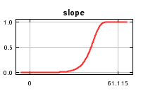
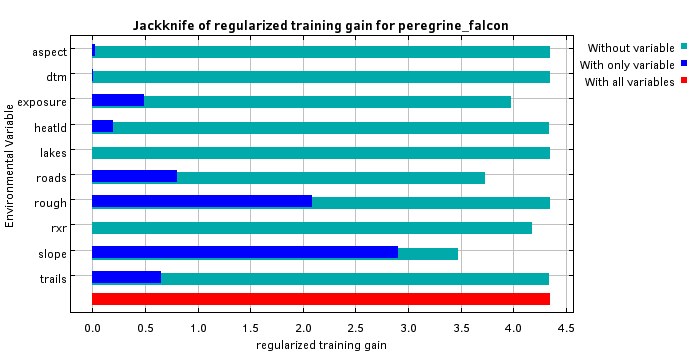
The slope had the highest contribution and strongest predictive value among all of the variables with a moderate positive sigmoidal response as slope increased, and the largest decrease in gain after removal from the model (fig. 2,3). Given the preferred nesting habitat is on cliff faces this makes sense (Barnes 2011, Comrack and Logsdon 2008).
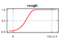
The roughness index showed a strong positive sigmoidal response as roughness increased( fig. 2, fig.4). Basically this is a measure of topographic heterogeneity and given that cliff faces are atypical for the area I would expect areas with higher heterogeneity to include greater slope variation. The removal of the variable from the model had little affect on the gain and is therefore highly correlated with other variables (fig. 3).
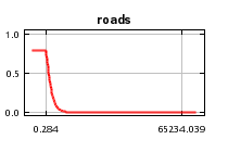
For roads there was a moderate negative sigmoidal response curve as distance from roads increased (fig.2, fig. 4). Roads do show a strong positive response to being in the model and show some response to their removal (fig.3). Though that may mean it is an important variable this is most likely the result of sample bias and more presence samples are needed to clarify the response. This is also where the understanding of Peregrine falcon behavior becomes important and an understanding of how the data was collected. The bias is most likely due to roads giving easier access to remote areas and therefore more sightings near roads. The subject matter expert (SME) who provided the presence samples did inform me that some raptors actually do have a positive response to roads due to greater availability of perches near an open area, and may even scavenge road kill.
For the wind exposure variable there was a weak positive sigmoidal response as wind exposure increased (fig.2, fig 4). This is most likely due to correlation between slope and wind exposure, there was only a small decrease in gain as the wind exposure variable was removed from the model (fig 3 jack). Peregrine falcons prefer very steep sloped nesting sites, generally on cliff faces, this habitat choice generally indicates a greater wind exposure (Barnes 2011, Comrack and Logsdon 2008).
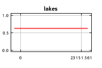
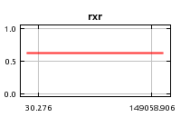
For the railroads variable there was a positive effect that did not change over distance (fig.2). After examining the jackknife test the variable on it's own has no value and should be removed from the model (fig. 3).
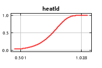
The model has a very weak positive sigmoidal response to an increasing heat load index (fig.2. fig.4). Heat load index is a relative measure of how much heat a particular area may retain based on hours of sunlight while also taking into account aspect, as in southwestern aspects will generally retain more heat than all others (Evans et. al. 2014).
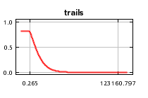
For the trails variable there was a very weak negative sigmoidal response as distance from trails increase (fig.2, fig. 4). This is most likely a artifact of sampling bias given sample sites are more often near roads and trails given ease of access. Given that the gain does not decrease after exclusion form the model more presence samples are needed to clarify the response (fig. 3).
Conclusions
Unfortunately this model has low predictive value due to the elimination of many locality data points as a result of quality control. However stricter quality control standards are now being implemented for data collection in the Shasta-Trinity National Forest and the variable layers still hold value having been created and processed for habitat modeling. If a protocol or structured survey methodology is implemented in the STNF with modeling in mind then additional locality points will improve the accuracy of this model. This project makes no attempt to assess the accuracy of the model. A lot of models base there data points on presence or observation points of a species, as does this model. The difference for this model is the unit of study is the nest locality, not where a peregrine falcon is observed. What this means is naturally this model will be derived from fewer presence points because there are always going to be fewer nest localities as opposed to observations of individuals anywhere spatially. In the future there are steps that can be taken to fine tune this model such as using environmental variable data for the species over a much larger portion of the range and use a portion of it as background samples. Additional suitable variables will continue to be added as they are found, and others rejected as the analyses dictate. Developing and improving this model will be an ongoing iterative process as I learn new techniques, as additional research is published, and as I develop a greater understanding of the subjects encompassing habitat modeling and prediction.
Acknowledgements
I would particularly like to thank the
following people and entities for there support and
advice on this project:
The US Forest Service and William Thein for providing me with the nest site locality data.
Paul Veisze
Marvin Castenada
I am sure there are many other people that have helped me along the way with this project and though I may have forgotten to include you I thank you for your help and support as well.
I would also like to credit free and open source projects such as SAGA GIS, Maxent, and Linux (Solus OS) that played an important role along the way and saved my bacon many times.
Most importantly I would like to thank my fiancée Paula Carrico for all of her support along the way. She is always there to lend an ear and her prespective, and do other important things like keep me from killing my computer.
References
Barnes, Joseph Graham,(2011) "An
Ecological study of peregrine falcons (Falco
peregrinus) at Lake Mead National Recreation Area,
2006-2010" .UNLV
Theses/Dissertations/Professional
Papers/Capstones.Paper 1028.
Brambilla M, Rubolini D, Guidali F, (2006) Factors affecting breeding habitat selection in a cliff-nesting peregrine Falco peregrinus population. J Ornithol 147:428-435
Comrack, L.A. and R.J. Logsdon (2008) Status review of the American peregrine falcon (Falco peregrinus anatum) in California. California Department of Fish and Game, Wildlife Branch, Nongame Wildlife Program Report 2008-06. 36pp+ appendices.
Conrad, O., Bechtel, B., Bock, M., Dietrich, H., Fischer, E., Gerlitz, L., Wehberg, J., Wichmann, V., and Böhner, J. (2015): System for Automated Geoscientific Analyses (SAGA) v. 2.1.4, Geosci. Model Dev., 8, 1991-2007, doi:10.5194/gmd-8-1991-2015.
Evans JS, Oakleaf J, Cushman SA, Theobald D (2014) An ArcGIS Toolbox for Surface Gradient and Geomorphometric Modeling, version 2.0-0.
Available: http://evansmurphy.wix.com/evansspatial. Accessed: 2015 Dec 2nd.
Hernandez, P. A., Graham, C. H., Master, L. L. and Albert D. L. 2006. The effect of sample size and species characteristics on performance of different species distribution modeling methods. Ecography 29: 773-785.
Phillips, Steven J., Miroslav Dudík, Robert E. Schapire. [Internet] Maxent software for modeling species niches and distributions (Version 3.4.1). Available from url: http://biodiversityinformatics.amnh.org/open_source/maxent/. Accessed on 2017-12-9.
Duan, Z., Zhao, D., Zeng, Y., Zhao, Y., Wu, B., & Zhu, J. (2015). Assessing and Correcting Topographic Effects on Forest Canopy Height Retrieval Using Airborne LiDAR Data. Sensors (Basel, Switzerland), 15(6), 12133–12155. http://doi.org/10.3390/s150612133