Malibu Creek State Park Landcover Analysis

by Caitlin McHugh

w1946602@apps.losrios.edu

American River College

Geography 350: Data Acquisition in GIS

Fall 2021

Abstract

I completed a Landcover Image Classification and generated a NVDI image from NAIP imagery of the Malibu Creek State Park to show the impact of the 2018 Woolsey fire for this project. The imagery was taken on 07/22/2018 (before the fire) and after the fire, 05/15/2020. This region experienced a post-fire bloom of invasive plants that grow fast, outcompeting the native plants. Through this image classification, I found that there was a massive regrowth of mustard and grass in the regions that experienced fire. These invasive plants are also spreading beyond the burn area and outcompeting the native chaparral, shrubs, oaks, and sycamore trees.

Introduction

The Woolsey Fire ignited on November 8, 2018 and devastated the counties of Ventura and Los Angeles, burning 96,949 acres of land and destroyed 1,643 structures. This fire burned a portion of the Malibu Creek State Park and the surrounding area of Malibu and irrevocably altered the vegetation and landscape. These plants, like mustard and grass, endanger the remaining shrubs, trees, and chaparral that made it through the first fire. I chose this specific region inspired by an article detailing the post-fire bloom that the park experienced, made up of invasive plants that grow fast, outcompeting the native plants. These invasive non-native plants accelerate fires without adding any useful biologic function to the area. I completed a Landcover Image Classification and generated a NVDI image from NAIP imagery of the Malibu Creek State Park for this project to identify the landcover and analyze the post-fire regrowth. The identification of these invasive weeds are important to create plans for removal and also for slope stability. This invasive vegetation is a huge hazard that needs to be addressed.

Background

Three quarters of the Malibu State Parked burned in the Woolsey Fire. This article details the post-fire bloom that the park experienced, made up of invasive plants that grow fast, outcompeting the native plants. These plants, like mustard and grass, endanger the remaining shrubs, trees, and chaparral that made it through the first fire. These invasive non-native plants accelerate fires without adding any useful biologic function to the area. This article educated me on the long-term effects of fire on the California landscapes, although learning more about devastating fires can be difficult.

Methodology

These are the steps I took to complete my image classification and NVDI image generation. I will include hyperlinks as a resource as well as citations in the references section.

1. Obtain Data:

Downloading from the USGS Earth Explorer

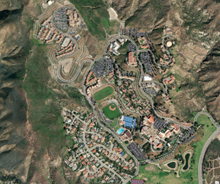
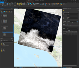
a. I first obtained data from the Landsat 8 data set. I found many dates of images for the area. However, this data did not have a high resolution (thirty-meter cell size) for the park and the image classification was hard to do. I included an example below of Landsat8 imagery and the Google Earth satellite imagery. I also ran into some issues with cloud cover with the imagery as well.

Lansat8 Imagery:

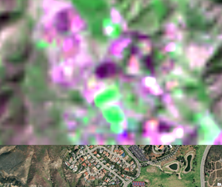
Google Earth:

Cloud Cover:

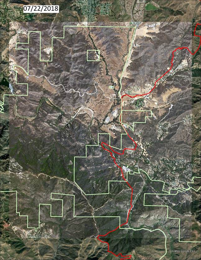
b. I found better data from the NAIP that had a one meter cell size. I downloaded this directly from the USGS. The imagery was taken on 07/22/2018 (before the fire) and after the fire, 05/15/2020.

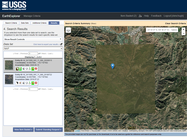
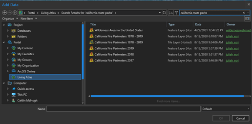
c. I obtained the fire perimeter and the state park boundaries from Living Atlas. I queried Malibu Creek state park and Woolsey Fire in the properties of the feature layer.

2. Preparing the Image for Image Classification

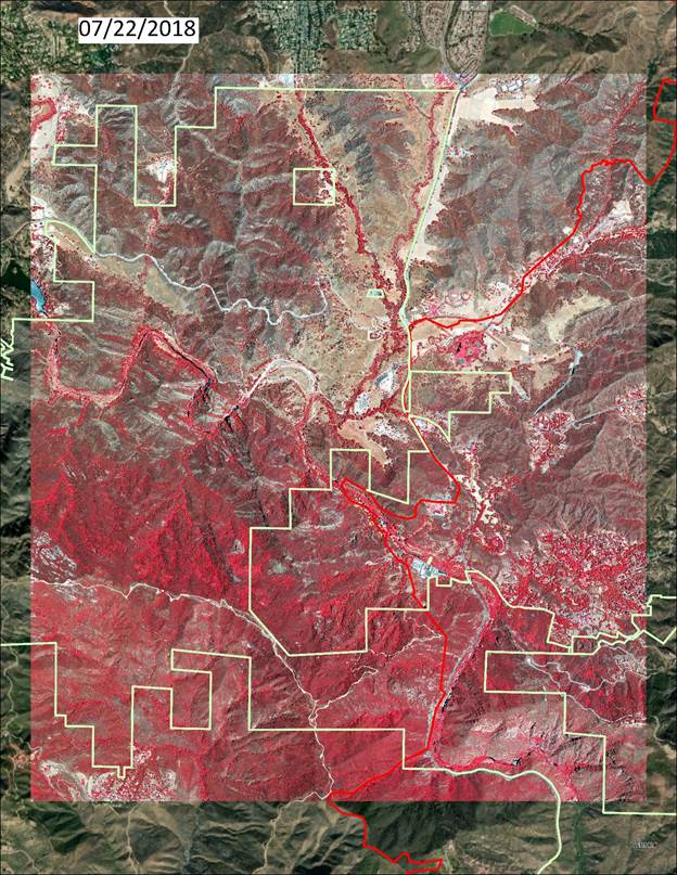
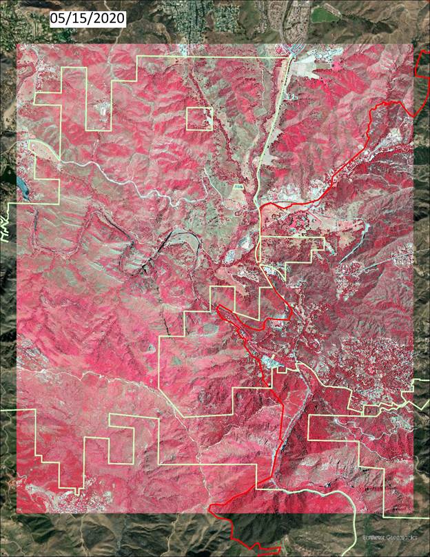
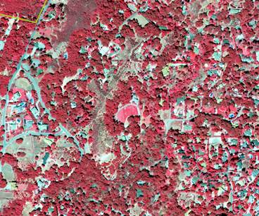
a. Changing the image from the natural color to Color Infrared (CIR)

Using a guide that I found on the USDA website and this tutorial, I colorized both images in CIR, also called a false color image.

According to the USDA Guide on NAIP Four Band Digital Imagery:

"If an image is created with the red (wavelength) band as band 1, green as band 2, blue as band 3, and near infrared as band 4, a natural color display on the computer screen would be set up with the red (display) channel as band 1 (red), green channel as band 2 (green), and blue channel as band 3 (blue). CIR would be set up with the red channel as band 4 (NIR), the green channel as band 1 (red) and the blue channel as band 2 (green). Band 3 (blue) is omitted."

I exactly did this by modifying the symbology of the raster in the symbology pane to Red (Band_4), Green (Band_1), and Blue (Band_2).

The image shows up like this:

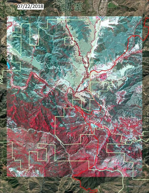
b. Segmenting the Image

I used the image classification tool to segment the CIR image, similar to the image segmentation in the Image Classification Module for GEOG 342.

The output looked like the image below.

3. Image Classification

Using the Segmented Images and the CIR images, I began the image classification Process

I used the steps outlined in the Image Classification Module and on the esri website:

a. Segment the image (image segmentation (Covered above)

b. Configure classification method (in this case Supervised (based on objects, object based))

c. Create training samples from the segmented output

d. Train the classifier

e. Run the Classification (i.e. Classify/Categorize the raw pixels into land cover types).

f. Merge Classes (e.g. more specific class to general classes)

g. Reclassify problem classes

h. Generate the final land cover classification image

I will detail those steps here for the Classification Wizard:

a. Segmented the image (Covered above).

b. Configured classification method

Classification Method: Supervised

Classification Type: Object Based

Classification Schema: NLCD2011 (National Land Cover Dataset 2011).

Segmented Image:

Training and Reference were not filled in.

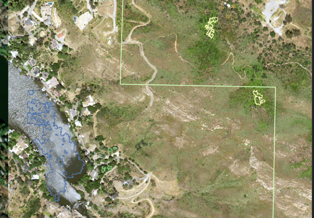
c. Create training samples from the segmented output

You can see the corresponding colors of types of land in the images. I added a class called "Mustard" to the 2020 image to indicate where the plant was visible. Here are some examples of the training samples I used:

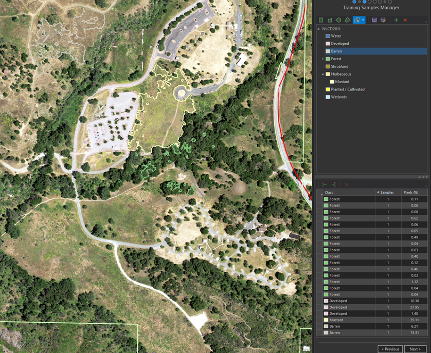
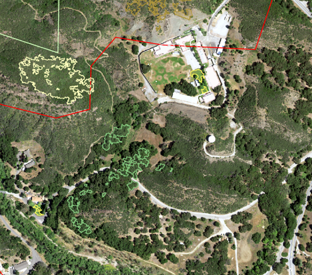
The mustard was particularly bright, which is why I gave it it's own class. All of the bright green here is mustard.

When creating training samples, I used the natural color imagery mostly. The images were so clear and distinct that it made it easy to choose the correct class. I did use the definitions of the NLCD classification scheme to help decide what to class.

Hint: I used the C key to toggle around while choosing training samples to avoid having to go back and forth from the map and imagery pane. This is a simple keyboard shortcut to make life easier in ArcGIS Pro in any mode.

d. Train the classifier

I used the defaults and the Support Vector Machine classifier. The run time took about 2-3 minutes.

The preview looked pretty good! I used this preview to "reclassify" any problem areas by toggling back and forth while going back to the samples training manager rather than use the reclassifier. I found this to be easier than using the reclassifier.

e. Run the Classification

I was happy with a closer inspection of the classified images, so I did not need to merge classes or reclassify problem classes.

[Skipped steps f & g that could be completed if not satisfactory]

f. Merge Classes

g. Reclassify problem classes

h. Generate the final land cover classification image

I changed the color scheme of the classified image to have more visible differences in the classified image.

The final land cover classification image is in the final images section. Here is a preview:

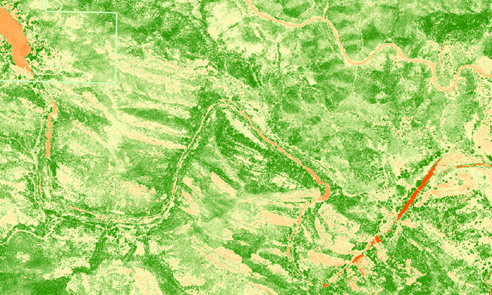
4. Normalized Difference Vegetation Index (NDVI) Image

I used the Normalized Difference Vegetation Index (NDVI) Image Colorization tool in ArcGIS to get these images from this guide.

The formula is (NIR – Red)/ (NIR + Red), where NIR is the Near Infrared channel, and Red is the Red channel.

For the Visible band, I used band 1 (Red) and the Infrared Band in NAIP imagery is band 4.

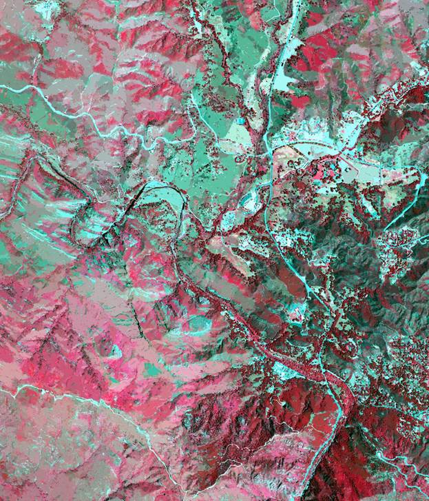
Here is an example of the colorized NVDI:

Results

Final Imagery

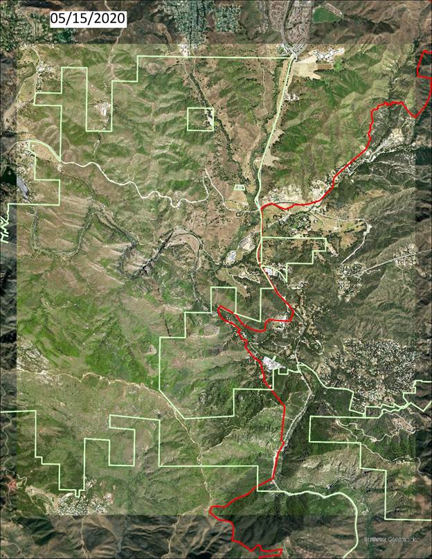
Natural Image

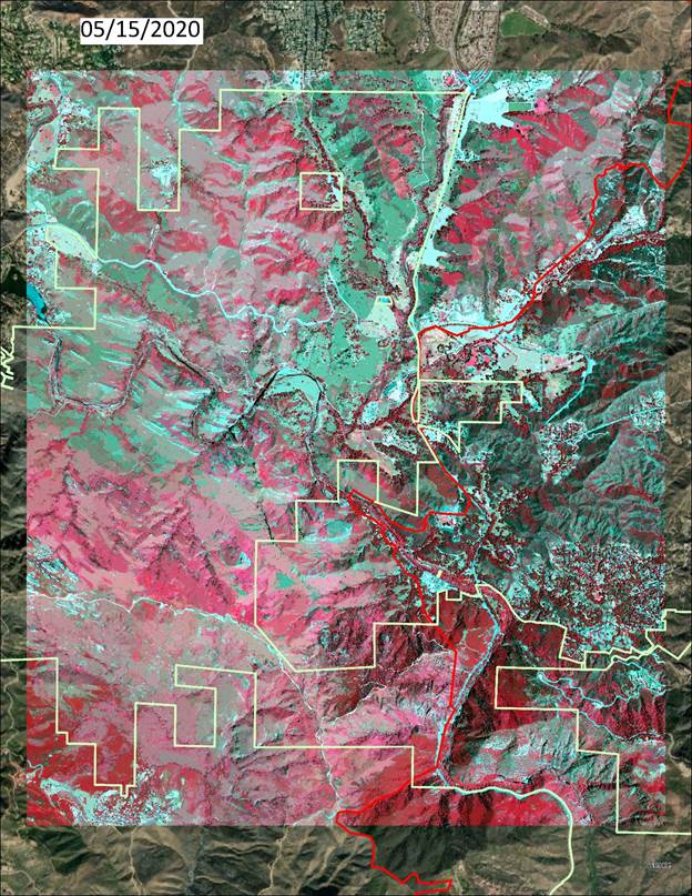
CIR Image

Segmented Image

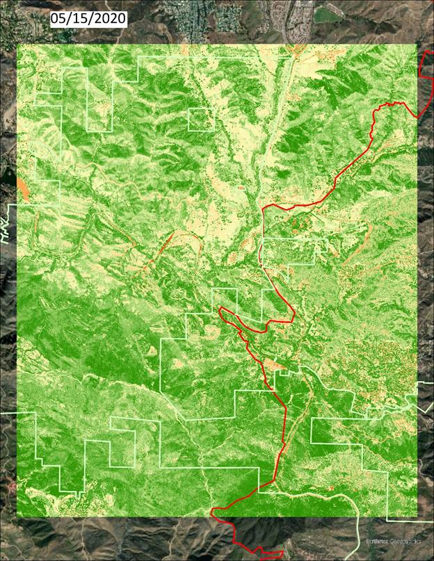
NVDI Image

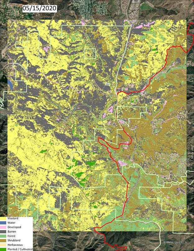
Classified Image

Natural Image

CIR Image

Segmented Image

NVDI Image

Classified Image

Analysis

What does the Output Imagery Show?

2018 Image 2020 Image

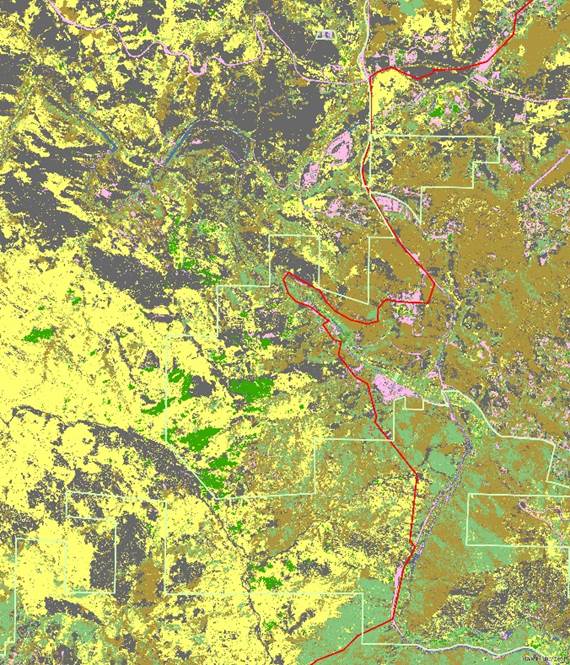
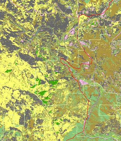
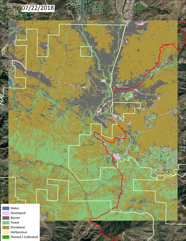
Landcover Classification Image:

When I classified the mustard as a class, I wanted to highlight just how much the landcover had changed. The mustard growth was consistent with the fire boundary. The fire took place in the western portion of this image, up to the red line. The mustard had even visibly extended beyond this boundary. Grass has also grown in burned areas (shown in bright green).

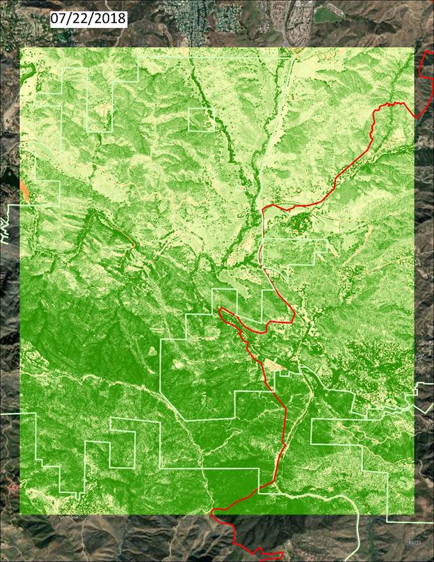
What does the output imagery show?

2018 NDVI 2020 NDVI

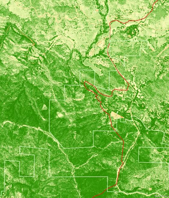
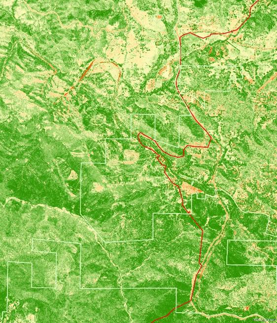
This image shows the mustard and grass flourishing in the places that it has taken over or regrown in burned areas.

Conclusions

The vegetation cover has had massive changes since the 2018 Woolsey Fire. This shift from drought resistant chaparral, shrubs, and forests to mustard leaves the area susceptible to fire again as well as landslide. With more fire, more non-native vegetation will take over and increase the risk of fire. There is a need to help regrow native vegetation to prevent an increase in fire danger.

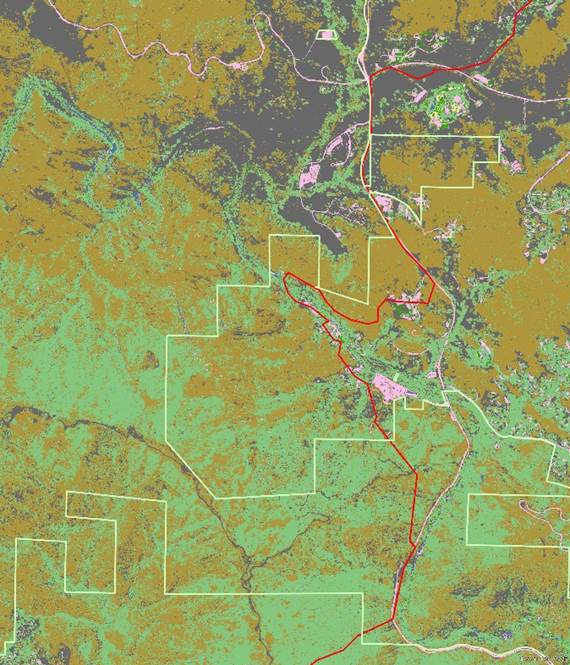
The loss of the shrubs and chaparral is apparent in the 2020 photo and the takeover of mustard and grass has prevented the slow rebirth of the native plants. You can see that there was less loss of shrubland and forest on the southeast portion of the image where the fire did not burn. However, the mustard is creeping in and stifling the native growth. Initially I thought the green planted/cultivate areas in the center of the image were misclassified, but upon closer inspection this region was actually grass growth that appeared very similar to the cultivated lawn grass that I trained the image to. These grassy areas are also non-native growth that are more susceptible to fire.

Overall, this image classification was very successful with some reclassifying. Because the image had such a high resolution, I spent a lot of time selecting individual houses, shrubs, roads, and trees to train the classification tool. I spent a quite a few hours training each image, but it was time well spent while inspecting the final classification. I did not expect to so clearly see the mustard and grass invasion from satellite imagery or have an classification scheme that was able to identify these non-native plants. I also did not expect to see how badly this invasive species had taken over.

References

Cart, Julie. “California Blooms Again after Last Year’s Fires—but It’s Not All Good - CalMatters.” CalMatters, CalMatters, 1 Mar. 2019, https://calmatters.org/environment/2019/02/californias-charred-hills-bloom-again-not-all-good/.

Four Band Digital Imagery INFORMATION SHEET. United States Department of Agriculture, 2013, https://www.fsa.usda.gov/Internet/FSA_File/fourband_infosheet_2012.pdf.

“National Land Cover Database 2019 (NLCD2019) Legend Multi-Resolution Land Characteristics (MRLC) Consortium.” Multi-Resolution Land Characteristics (MRLC) Consortium Multi-Resolution Land Characteristics (MRLC) Consortium, Multi-Resolution Land Characteristics (MRLC), 2019, https://www.mrlc.gov/data/legends/national-land-cover-database-2019-nlcd2019-legend.

“NDVI Colorized Function—ArcGIS Pro Documentation.” Pro.Arcgis.Com, ESRI, https://pro.arcgis.com/en/pro-app/latest/help/analysis/raster-functions/ndvi-colorized-function.htm. Accessed 10 Dec. 2021.

“The Image Classification Wizard—ArcGIS Pro Documentation.” Pro.Arcgis.Com, ESRI, https://pro.arcgis.com/en/pro-app/latest/help/analysis/image-analyst/the-image-classification-wizard.htm. Accessed 10 Dec. 2021.

Wasser, Leah. “How to Open and Work with NAIP Multispectral Imagery in R Earth Data Science - Earth Lab.” Earth Data Science - Earth Lab, Earth Lab, 22 Feb. 2017, https://www.earthdatascience.org/courses/earth-analytics/multispectral-remote-sensing-data/naip-imagery-raster-stacks-in-r/.