Title
On Historical Earthquake Characteristics Along the Bitterwater – Parkfield Segment of San Andreas Fault

Author Information
Mojtaba Mostajaboddavati
American River College, Geography 350: Data Acquisition in GIS; Fall 2021
4700 College Oak Dr, Sacramento, CA 95841
MojtabaMostajab@gmail.com

Abstract
In this paper we report historical earthquake characteristics repeatedly occurred in vicinity of the San Andreas fault system. We also try to investigate why they show similar attributes and why they are repeated and search for new hidden characters. We used GIS technology as a convenient research tool and as a powerful data visualization for Earthquake Prediction (EP) purposes. Tectonic earthquakes are caused by uniform relative motion of tectonic plates and happen in two plates' boundaries, which are called faults. If noncomplex boundary contact area and relative velocity of plates remain fixed, in absence of perturbative agents, reoccurring identical events is expected. Simply because energy budget and involving mechanical properties of materials remain uniform. In California, the San Andreas Fault (SAF) zone has been a very significant source of major earthquakes. In almost a century, from 1812 to 1906, it generated four major earthquakes of magnitude 7 or larger in two pairs on two major segments of the fault. During last two centuries, in central portion of the SAF, called Bitterwater - Parkfield Segment (BPS), six moderate earthquakes occurred. These events have similar characteristic. Three of these events have instrumental seismograph recordings with very similar signatures. This similarity motivated scientists to propose to set up a natural earthquake laboratory for EP by installing measurement equipment around BPS. We calculated vertical component of tidal acceleration at points and occurrence times for seven events, a trend for tidal triggering is observed. We used GIS technology as a convenient research tool and, at the same time also a powerful data visualization for EP purposes. Based on the expertise from GIS technology, in science of EP we really need is a Geophysical Information System (GPIS) which can integrate geophysical, geological and geographical information. In GPIS, solid earth tides for earth’s crust are automatically calculated. Finite element approach for crust stresses and deformation is included in that software.

Introduction

Earthquake Prediction (EP) continues to be one of scientific controversial topics in geophysics for more than at least a century. Some scientists maintain their hopes that with more earthquake precursors data we will eventually be able to forecast future events related to a well-known simple geometry fault system. Others, argue that an earthquake event is an emerging phenomenon from a complex nonlinear mechanical system which is very sensitive to fine perturbations, to its fault history and/or to initial conditions. They conclude that earthquakes are inherently unpredictable, and precursors are not universally belonged to series of cause-and-effect sequences connecting to earthquakes.
There are several earthquake precursors reported in different geographical regions over years, although before a specific tectonic earthquake a few, or even all, of them may not show up. Tectonic earthquakes, different from volcanic earthquakes, originate as a result of relative motion of large adjacent pieces of crust, each called a plate. When two plates collide with an average relative velocity of several millimeters per year, they both deform and store energy in their deformed parts just like a compressed spring, but in three dimensions. The amount of deformation, which depends on mechanical properties of materials involved, is a physical quantity called strain; it is simply relative displacement of particles of the deformed body (rock). Stress is another physical quantity which quantifies the internal forces between particles of a mechanical continuum. For a given single and simple (not a multilayered) boundary, a certain relative velocity of the plates and a fixed contact area, when friction between involving plates prevents slow but continuous slipping, energy accumulates until internal forces are about to overcome frictional forces. During this process, when deformation takes place, microcracks are created within rocks in and around the boundary. When the fault is in breaking threshold state, even small changes to accumulated stress can trigger a sudden rupture. Solid earth tides due to moon and sun, static or dynamic stress transfers from near or remote earthquakes, sudden and large changes to atmospheric pressure, sea or ocean tides, electric or magnetic forces between plates and external or internal electric charges in the atmosphere and any sudden load or unload due to snow, rain or flood may trigger earthquake to happen when stress is in near break threshold.
Let's assume that relative velocity of plates for a given fault and its contact area are fixed and don't change after an earthquake originated from this fault system. In the absence of any perturbative agent mentioned above, fault geometry, mechanical properties of fault material and stored energy budget determine when frictional is overcomed and hence earthquake happens. According to this simplified scenario earthquakes related to this fault should be repeated regularly, if our assumptions are valid. Furthermore, in this situation all these earthquakes shall be identical, the same magnitude, similar waveform, the same motion etc. If the assumptions are not completely valid, meaning earthquakes change the fault system somewhat, the repeated earthquakes are somewhat similar but not identical to each other. So, study of repeated nearly identical earthquakes helps to understand earthquakes' processes.

Background

Geological evidences indicate that San Andreas Fault System (SAFS) started moving about 28-30 million years ago and has horizontally slipped a total of 300 to 350 km since it began moving. The SAFS is the main part of the boundary between the Pacific tectonic plate on the west side and the North American plate on the east side. The SAFS consists of a main fault, that is San Andreas Fault (SAF), and many sub-parallel faults that all together take up the motion between the two plates. In northern California, there are several faults, including Hayward, Calaveras, as well as Northern San Andreas Fault. In the southern section, the system is wider encompassing Southern San Andreas, San Jacinto and other faults in Los Angeles area. In central part of the system there are some other fault branches. A portion of SAF near Parkfielf, is called Bitterwater - Parkfield Segment (BPS).
The relative motion between two tectonic plates is 50 mm/year, but this rate is distributed amongst all faults in the system. Each fault in the system is a boundary between two blocks. The motion of each block can be measured by analyzing GPS data. The faults themselves are stuck, but move where there is a high magnitude earthquake. Some faults creep, but most are locked. As explained, an earthquake occurs when the force from deformed stressed material of moving plate overcomes the friction causing the plate boundary edges to stick. The plate slowly moves all the time, but edges ( i.e. faults) move in fits and starts.


Bitterwater - Parkfield Segment 
of San Andreas Fault System in central California is shown


Figure 1. Bitterwater - Parkfield Segment of San Andreas Fault System in central California is shown. All historical earthquakes related to BPS (dashed area) are shown. Some other earthquakes in the region are also indicated.

The epicenters of mainshock and two foreshocks in 1857 were probably located on the San Andreas fault near Parkfield. After 1957, earthquakes with main shocks of magnitude 5.5 or higher have occurred near Parkfield on 2 February 1881, 3 March 1901, 10 March 1922, 8 June 1934, and 28 June 1966. The time interval between two consecutive earthquakes are remarkably uniform, with a mean interval of 21.9 ± 3.1 years. The occurrence time earthquakes is ploted as a function of order number in Figure 2 with Bakun’s linear regression equation T = 21.7I + 1836.2.

this is my big green map


T. R. Toppozada et al investigated and compared 1857, 1881 and 1901 seismicity regions and concluded these earthquakes have similar characteristics, their epicenters are probably close to WPS, their magnitudes and ground motions are similar. East-west components of waveforms for 1922, 1934 and 1966 earthquakes from De Bilt station in Europe are shown and compared in Figure 3. The similarities are clear, indicating they originated from nearly the same point.

this is my big green map


this is my big green map


Figures 4 and 5. The P-wave signals show the north-south components for (A) the Parkfield main shocks and (B) foreshocks. The 1934 and 1966 are shown by dashed and solid traces, respectively. Amplitude scales refer to the original seismograms. (C) Pn spectra for two main shocks. (D) Pn spectra for the 1934 foreshock (dashed traces) and an earlier 1934 foreshock (solid traces). The similarities between compared spectra are clear.

this is my big green map


this is my big green map


this is my big green map


Discussion

Based on the our probable scenario or model mentioned above, it can be concluded that the assumptions we stated are nearly valid and, thus, we may expect these six quakes should be outcome of nearly identical mechanical situations. So, we also expect that time intevals between these earthquakes should be nearly similar. But it is seen that 1934 event is about a decade early. We try to investigate possible explanations for this problem. It was mentioned previously that only in absence of any perturbative agent our expectations would come true. But all triggering mechanisms are present and in competition for their time dependent effectiveness priority order, thus cannot be ignored.
Let's note that there were three quakes recorded on 8th of June of 1934 in Parkfield area, which are Tabulated in Table 2. The location of these earthquakes are shown in Figure 6. Two earlier ones are next to each other, have shallow depths of 6 km and higher ml magnitudes, 5.09 for foreshock and 5.84 for the other. The epicenters of shallow quakes are placed in about 30 km northwest of the lower magnitude third one, with depth at 16 km. It is possible that the shallow events are related to a fault parallel to WPS with similar geometry. These two quakes redistributed stress and reduced stress in southeast of their epicenters; and hence triggering the third quake close to city of Parkfield. In this situation, some trigger mechanism activate the first two quakes and then stress drop triggers 4.8 magnitude deeper rupture. We will discuss the initial triggering process in some detail in following section.


this is my big green map


Figure 6.
Table 2.
IDDateTimeLatitudeLongitudeMagDepthRef
19340608043021210 1934-06-08T04:30:21.210Z 35.8705 -120.6936667 5.09 6 USGS
19340608044746900 1934-06-08T04:47:46.900Z 35.8463333 -120.6663333 5.84 6 USGS
19340608054200000 1934-06-08T05:42:00.000Z 35.8 -120.33 4.5 16 USGS

Methods and Results
There are many triggering mechanisms for earthquakes. As mentioned earlier, SAFS is the boundary of two plates. The motion of plates accumulate stress and deform crust. The plates are stuck at the boundary or faults, while they move and deform. The geometry of boundry is usually complex with many faults. The geometry of fault system is an important factor in some of triggering mechanisms. Due to solid earth tides, a time dependent deformation pattern is imposed on the fault geometry. If the fault system is on its critical state, when tidal deformation matches the fualt geometry, a rupture may happen.
There are times that time dependent deformation of crust tries to pull apart the plates, while some other patterns pushing the plates together. There are certain configurations of earth orientation, fault system geometry, moon and sun celestial coordinations which help the stressed and deformed crust to jamp like compressed spring. In this section, we presente the calculated vertical component of tidal force at epicenter of earthquakes related to WPS. These similar earthquakes happened in certain tidal time intervals, so there are similar triggering agents are in action. For each fault geometry, there are time characteristics when measured with a "tidal clock". We have calculated time varying vertical component of tidal acceleration (or force) for 12 hours before and after each earthquake and ploted them. Vertical axis is shown in arbitrary units. Earthquake time is set to zero.

001857"


001881.jpg


001901.jpg


001922.jpg


001934,jpg


001966.jpg


002004,jpg


It is seen from the plots, Parkfield earthquakes, including the 2004 quake, happened in time interval from about maximum high tide to low tide. This observation reduces the occurrence time interval by a factor of about half, when compared to random time distribution.


Comparing Tidal Plots


this is my big green map


Conclusion
Tectonic earthquakes happen mostly in boundaries of moving plates. In colliding process, while moving plates stick together by frictional forces in contacting surfaces, the moving plates themselves deform. The deformed portions of crust set up stress in all points of crust material. This process continues and, at some point, micro-cracks begin to form in mechanical weaker regions. More and more deformation takes place and more energy is stored in compressed material. Subsequently, there will be a state where frictional forces are about be equal to internal forces due to shape change. At this stage, a small perturbation can trigger the a rupture. Solid earth tides are always 
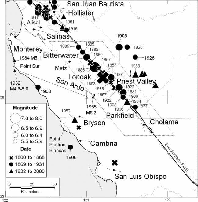
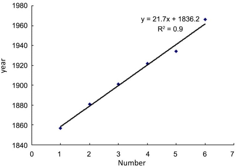
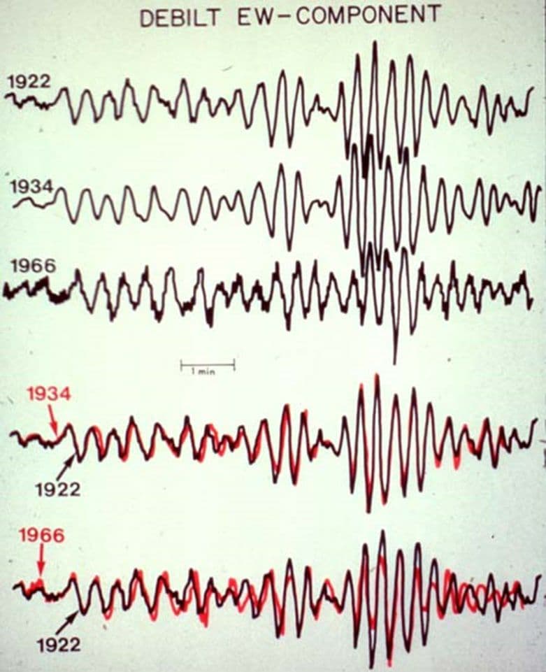
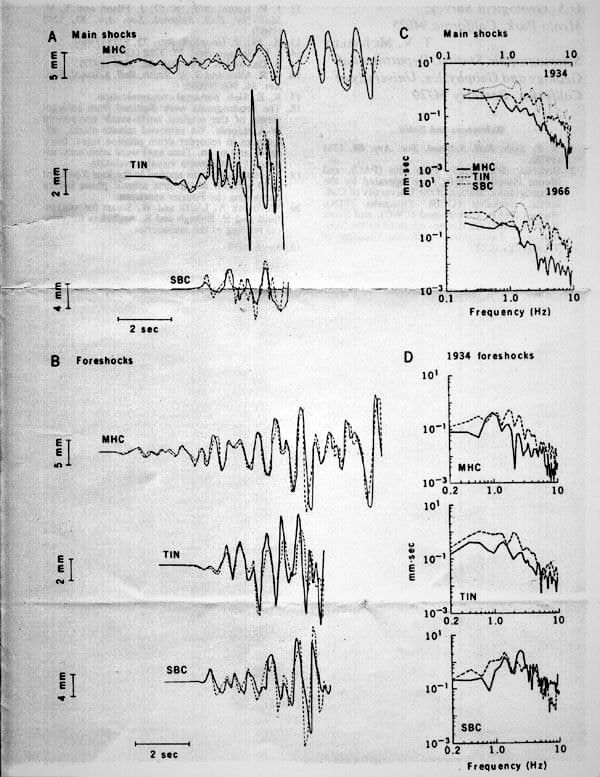
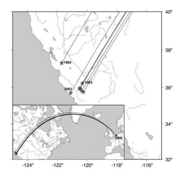
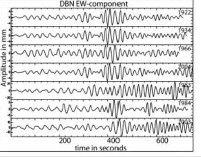
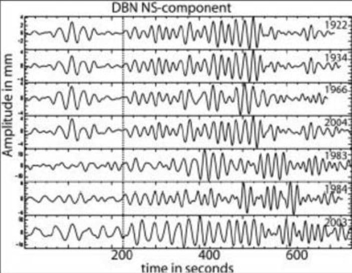
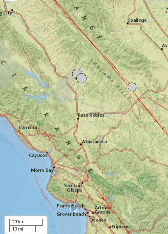
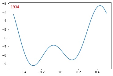
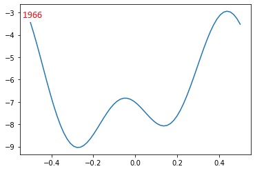
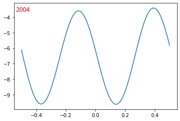
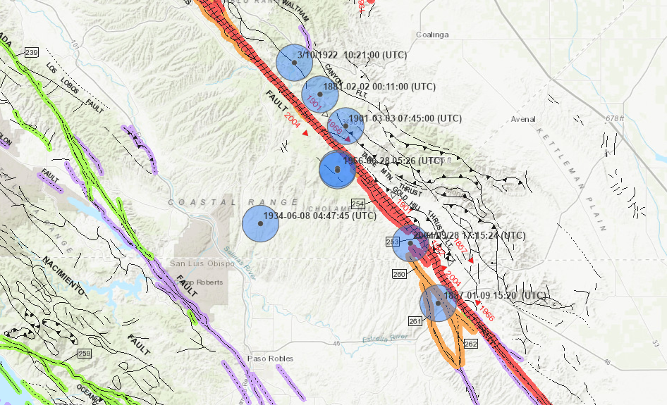
present as a periodical perturbative agent. In this research it is shown that similar earthquakes around Parkfield originated in the same fault system are tidally triggered. Breaking time intervals are between high to low tides. In these time intervals earthquakes were more likely to happen. We conclude that solid earth tides are an important mechanism to initiate earthquakes. This fact can be used in artificial intelligence earthquake forecast models for training purposes.

References
1) Bakun, W.H. and T.V. McEvilly, 1984. Recurrence Models and Parkfield, California, Earthquakes. J. Geophys.Res., 89, 3051-3058.

2) Bakun, W.H., B. Aagaard, B. Dost, W.L. Ellsworth, J.L. Hardebeck, R.A. Harris, C. Li, M.J.S. Johnston,J. Langbein, J.J. Lienkaemper, A.J. Michael, J.R. Murray, R.M. Nadeau, P.A. Reasenberg, M.S. Reichle,E.A. Roeloffs, A. Shakal, R.W. Simpson and F. Waldhauser, 2005. Implications for prediction and hazardassessment from the 2004 Parkfield earthquake. Nature, 437, 969-974. doi 10.1038/nature 04067

3) Dost, B. and H.W. Haak, 2002. A comprehensive description of the KNMI seismological instrumentation. KNMITechnical Report TR-245, 60pp.

4) Dost, B. and H.W. Haak, 2006.Comparing Waveforms by Digitization and Simulation of Waveforms for Four Parkfield Earthquakes Observed in Station DBN, The Netherlands.Bulletin of the Seismological Society of America, 96, S50-S55. doi: 10.1785/0120050813

5) Langbein, J., R. Borcherdt, D. Dreger, J. Fletcher, J.L. Hardebeck, M. Hellweg, C. Ji, M. Johnston, J.R. Murray, R. Nadeau. M. J, Rymer and J,A, Treiman. 2005. Preliminary report on the 28 September 2004, M 6.0 Parkfield, California Earthquake. Seismol. Res. Lett., 76, 10-26.

6) Michelini, A., B. De Seimoni, A. Amato and E. Boschi, 2005. Collecting, digitizing, and distributing historical seismological data. EOS transactions American Geophysical Union, 86, 261-266.

7) https://earthquake.usgs.gov/learn/parkfield/1922.php