Abstract

            A student geographic information systems project stays simple and sticks to the basics and still turns up amazing discoveries about the six supermarkets located in a defined urban area.

Foreword

           This semester I am taking two GIS courses which require projects. Early on, I settled on a supermarket study for Geography 9 (Introduction to GIS). As I proceeded to research and collect and manipulate data for the supermarket project, it occurred to me that this project involved a great enough investment in time and resources to apply toward the requirements of both Geography 9 and Geography 26 (Data Acquisition). This seems especially useful, because it gives me the opportunity to discuss in detail the gathering and processing of data for the Geography 9 supermarket project and the problems encountered along the way. These projects tend to complement each other. For Geography 26, I discuss both  the process and final product of data acquisition; for Geography 9, I briefly mention how I acquired the data and set up and demonstrate queries in ArcView of that data. The form for reporting on the two projects also lead to a useful divergence. The Data Acquisition course format is HTML (web page), while Geography 9 projects are to be submitted using a computer presentation format, such as Microsoft PowerPoint, and a demonstration in ArcView.

Introduction
                Data acquisition is a necessary prerequisite to any geographic information systems (GIS) project. This paper explores the process of accumulating data for a supermarket project conducted for my Geography 9 class (Introduction to GIS); the study would attempt to compare supermarkets based on the prices they charge their customers . The purpose of that project is to use the skills and knowledge learned during this, my first, semester in GIS. The general rule adhered to is summarized by the popular acronym KISS (keep it simple, stupid) with short but meaningful added in. The tasks involved are: 1. define the geographic area to be studied; 2. collect and process the relevant spatial data (which must be georeferenced); 3. design and gather the needed (nonspatial) attribute data needed for price comparisons between supermarkets;  4. draw conclusions, evaluate the study's methodology, and suggest additional steps to make the study more valid; and 5. present the project to a body of my peers for their evaluation and solicit from them suggestions which might improve the conclusions of the study. My approach to the problem is to use the data which are most easily and economically accessible and to avoid expenses which would bankrupt the project.

Background

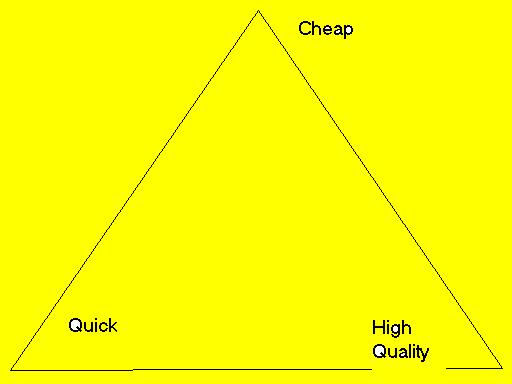
                A guiding principle throughout this project is that "data conversion, like so many things in life, quickly becomes an exercise in balancing trade-offs. Normally, you can only have two of the three coveted conversion characteristics -- good, fast, and cheap -- and must sacrifice the third. You can have data fast and cheap, but they're not going to be the best possible quality. You can obtain good data quickly, but they will be expensive. Or, you can have good data cheaply, but you're not going to get them very fast" (Hohl, 1998:8). This is illustrated in a model.  In any project, managers must select their two highest priorities; the third will result from that choice. For lack of a better term, I will refer to this as Hohl's Rule. My experience in this project led to a correlary for Hohl's Rule: the smaller the project, the more likely all three of these will be optimized. My project involves a limited amount of time, few dollars, and tentative results! This brings up a second guiding principle: when resources are limited, limit the scale of the project accordingly. Even large projects are often preceded by sample tests.
            The greatest opportunity in a project of this kind is to be able to use the techniques and express the concepts learned during a semester's toil. The quest for map data and the creation of a working map, as well as the less satisfactory sources and attempts cast aside, are valuable. My map production and other uses of ArcView were made possible by my previous experience with that application; but, mostly, I owe my instructors in Geography 9 and 25A/B/C (Dale Van Dam and Tom Lupo) and the publishers of Getting to Know ArcView GIS (1997). Instructors Van Dam and Paul Veisze (Geography 26) are responsible for my orientation in theories, concepts, and methods of data acquisition, manipulation, and analysis. My intention was to plow through the material covered in these courses to recall useful and relevant material that relates to this project and to record it for posterity. Murphy has struck again; his law is omnipresent and demands our attention, to forever play the "what if" game. "If something can go wrong, it will. And it will go wrong at the worst possible time." Ugly. But worth being aware of and now reminding me that time has played its course. DeMers has made a theme of the travel and adventure involved in the GIS experience. And this rings a familiar bell. Many times in our travels, we are just on a reconnaissance, finding places where we are not allowed to remain for long but jotting them down in our memories as sites to be revisited on the next best occasion. So be it with the current GIS efforts!

Methods

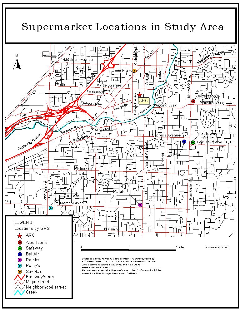
                Limit Geographic Area of Project.  The study area is limited to include the nearest supermarkets to the American River College vicinity. This area includes the area bounded by and adjacent to these major streets:  Auburn Boulevard, Madison Avenue, Manzanita Avenue, Fair Oaks Boulevard, Marconi Avenue, and Watt Avenue. Six stores represent major supermarket chains within the study area: Albertson's, Safeway, Bel Air, Ralphs, Raley's, and SavMax. (During the study, "Lucky married Albertson's." The store that started out as Lucky took on the Albertson's name as a result of a merger or buy-out. For simplicity's sake, that store is referred to as Albertson's throughout this paper. Ralphs is the "new kid  on the block"; it occupies the location of a former Albertson''s, closed due to the impending marriage to Lucky.)
                Spatial Data -- Primary Locations.  The primary geographic entities are the supermarkets. I collected GPS (Global Positioning System) data for each of these with a Garmin 12 XL unit. Tests with this unit by our class this semester indicate that it is reliable within certain limits, especially when selective availability is corrected for by using Garmin add-ons to make use of Coast Guard beacons. My data consisted of single points recorded in the supermarket parking lots, usually closer to adjacent streets than to the store itself. I did not correct for selective availability. When displayed with georeferenced maps of the area, the GPS positions appear to be "generally" accurate (looks right; certainly never more than 30 meters off; and never on the wrong side of the street). I also collected a GPS point on the American River College campus as a central reference point (the place to start to go shopping).  In making my final map for this project I made use of the "symbol placement compromise" by changing the locations of my GPS points; I made them more inaccurate by moving them so that they did not intersect the adjacent streets.
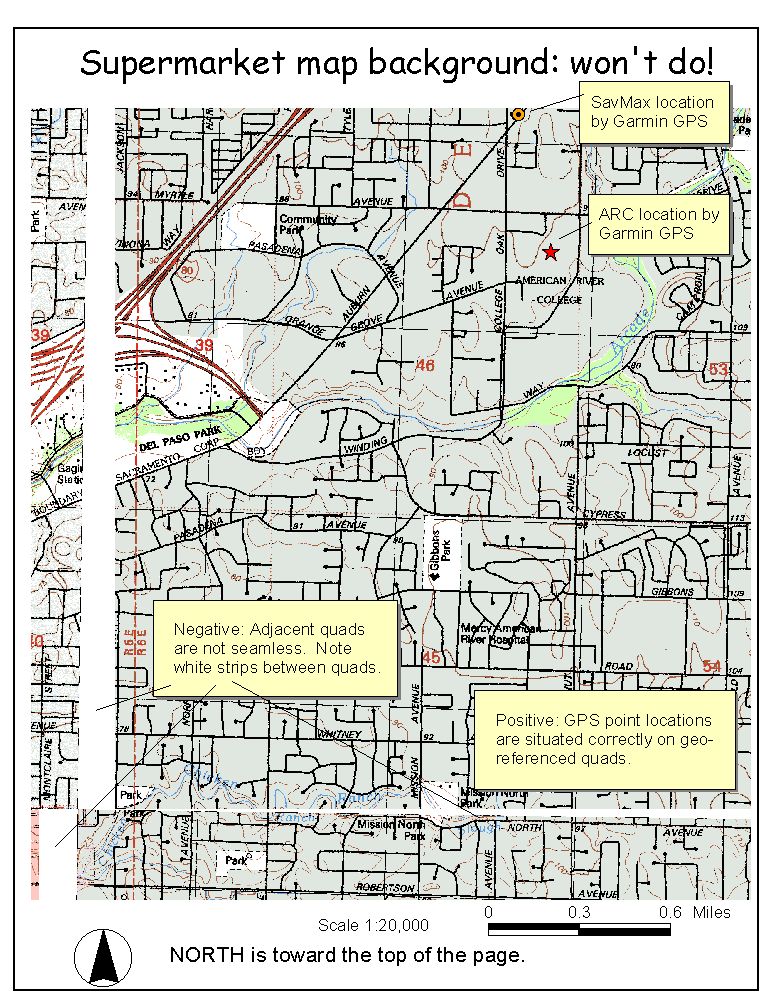
                Spatial Data -- Background.  For map background, I considered using files from Geography 26 data bank. Sheridan.bil image is an aerial photo which includes the project area; but it eats up a lot of computer space, comes up slowly, and I could not think of how it would be immediately useful. Sacramento.tif is a scanned map that also has a large size and too low of a resolution (large pixels). The set of scanned 1:24,000 quads at first appeared useful -- until I realized that they were not seamless along their edges. Seamless quads can be purchased locally at California Surveying and Drafting Supply (4733 Auburn Boulevard, Sacramento); they've got  MapTech (all of northern California for $319.00 but probably not georeferenced), DeLorme TopoUSA (at $99 for the whole country, probably not useful for GIS), and Garmin MapSource (1:100,000 quads that load into their GPS).  The best product I've seen is Sure!MAPS RASTER (seamless and georeferenced; available from GeoWarehouse on the internet at www.geowarehouse.com).  To stay within the budget (zero dollars), I decided against buying commercial products.
                Then I decided to digitize the freeways and major streets within the project area. This produced shapefiles for the freeways and major streets, making it unnecessary to use the georeferenced quads.  This worked out well.  But I found that I could improve the map by trashing what I had at this point and starting over, because I found the TIGER files for Sacramento County to be available from the SACOG (Sacramento Area Council of Governments) web page (http:\\www.sacog.org). My project is projected in Teale Albers, and the SACOG TIGER files are unprojected Lat/Lon. I was able to build a Teale Albers projection of the SACOG TIGER files in Arc View. ArcView includes an extension for projecting vector files. It is not loaded in the ArcView Extensions until the user moves it (prjctr.avx) from esri\av_gis30\arcview\samples to esri\av_gis30\arcview\ext32. 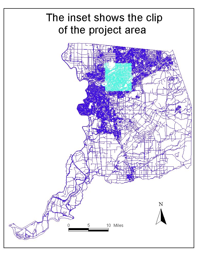After projecting the county TIGER shapefile to Teale Albers,  I clipped the project area from it, using the rectangle graphics tool, "Select Features from Graphics" button, and Theme|Convert to Shapefile in ArcView. MyClip shows the progress to this point.
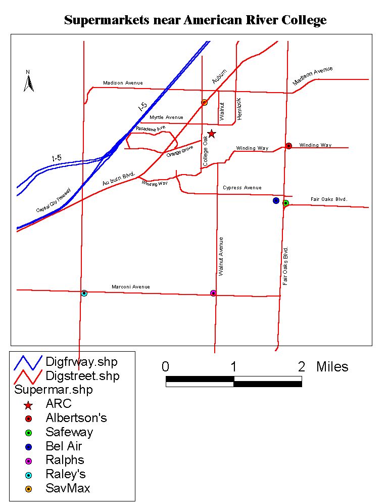
                I then worked with the TIGER clip of the project area to select the major geographic features. Within ArcView, I used the Query Builder and Theme|Convert to Shapefile to create themes for freeways, major streets, and creeks. To the view, I then added the Locations by GPS theme. A little more editing and adding symbology resulted in the final map layout for the project:
                Time Frame.  Data were collected during the period October 15 through December 12, 1999.
                Data Collection Intervals.  My intention was to revisit each store once a week during the project's lifetime; however, it immediately became obvious that such an effort would exceed project resources. This resulted in a compromise, where I collected prices from a single store (Albertson's) over a period of six weeks and of all six  stores on two occasions, at the beginning and end of the project (referred to as Slice 1 and Final Slice and coinciding with supermarket weeks including October 15 and December 3). This gives us an idea of how the six stores compare at two slices in time and how prices change over time at a single supermarket. In this report, only the first slice is illustrated in order not to overwhelm the reader with charts.
                Grocery List and Shopping Cart.  I arbitarily selected 38 items from among four categores:  dairy, produce, grocery, and household. These included eggs, milk, cottage cheese, and yogurt; bananas, lettuce, cauliflower, and potatoes; bottled water, juice, coffee, vegetable oil, olive oil, ketchup, mayonaise, peanut butter, flour, sugar, macaroni, spaghetti pasta, spaghetti sauce, rice, pinto and black beans, corn flakes, raisin bran, and canned tuna; and, finally,  laundry detergent and toilet tissue. The choice of these particular items was mostly random, with a vague plan to cast a net somewhat widely. In some cases, specific brands were targeted (e.g., Wesson oil in 24 ounce size and 1/2 gallon size of Breyers Ice Cream). In most cases, I selected the lowest price brand that fitted the general description of the item (e.g., taking the lower price of Post or Kellogg's raisin bran).  Some items had to be dropped off the list when I found that one or more stores did not carry an equivalent item. I eventually made up a "shopping list" composed of one or more items from the grocery list. It was from this list (or cartful of items) that I compared supermarket prices. If you have Microsoft Excel, you can pull up a sample of one of the spreadsheets I used by clicking here. It shows Albertson's prices at Slice 1 and the Shopping Cart list.
                Data on Prices.  As expected, the acquisition of nonspatial data was the most time consuming. Early on I learned to empathize with and admire those valient clerks who persevere and serve with wonderous smiles, as they ply their 8-to-9 hour work day over those hard concrete floors. To collect comparative price data, I prepared a hardcopy form with a list of 38 grocery items.  An entire day (10/15/99) was required for data collection during Week 1; subsequent pricing visits required a minimum of 30 minutes in the store (not counting travel time).  An additional 30 minutes or so would be required to enter the data in three separate Excel spreadsheets for each visit.
               Attribute Table.  I brought up the View in ArcView, selected my Locations by GPS theme, and brought up the attribute table for that theme. I edited the table to include an additional field, my key field, for each of the located points.
               Related Tables.  One of my goals was to build a database which would include a number of different tables with information about the supermarkets (address, phone number, etc.) and their prices.
               Charting Prices.  I constructed charts in ArcView to compare prices.
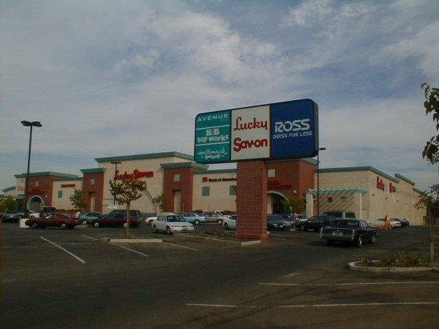
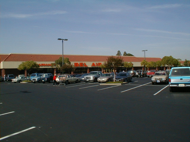
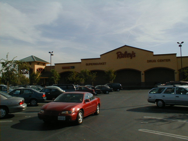
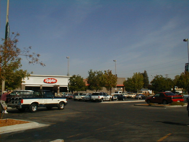
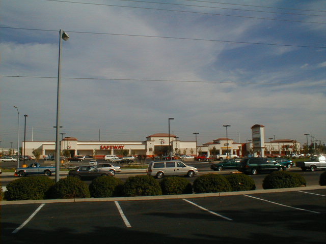
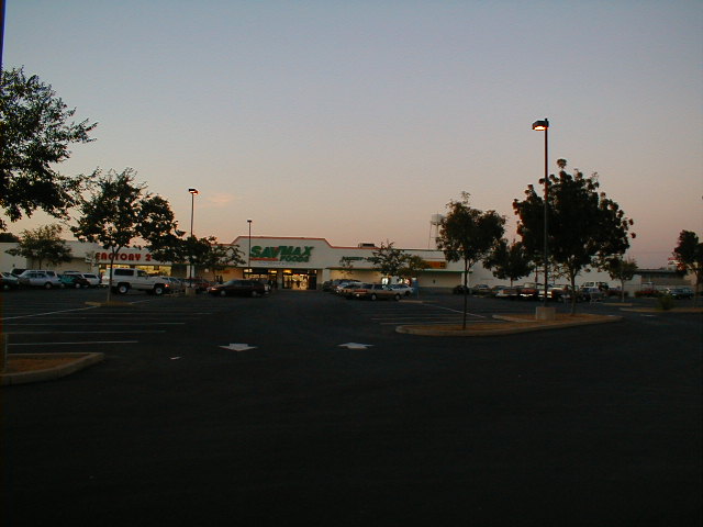
                Photographs.  I took digital photographs of each supermarket. In most cases, the photo is taken in the parking lot at the location where the supermarket GPS point was recorded.

Results

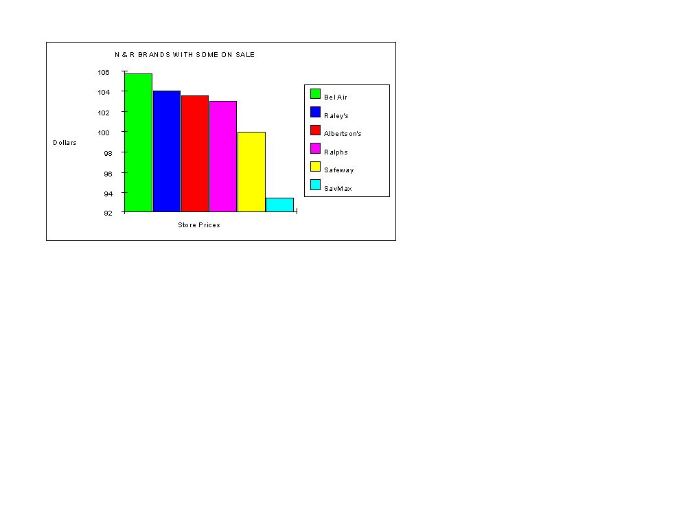
                Summary.  Slice 1 of the study shows a consistent pattern: highest prices were at Bel Air and lowest prices were at SavMax.  One surprise was that there was such a wide disparity between Shopping Cart prices for Bel Air and Raley's, two affiliated supermarkets. That led me to collect prices for a second slice at the end of the project's lifetime. 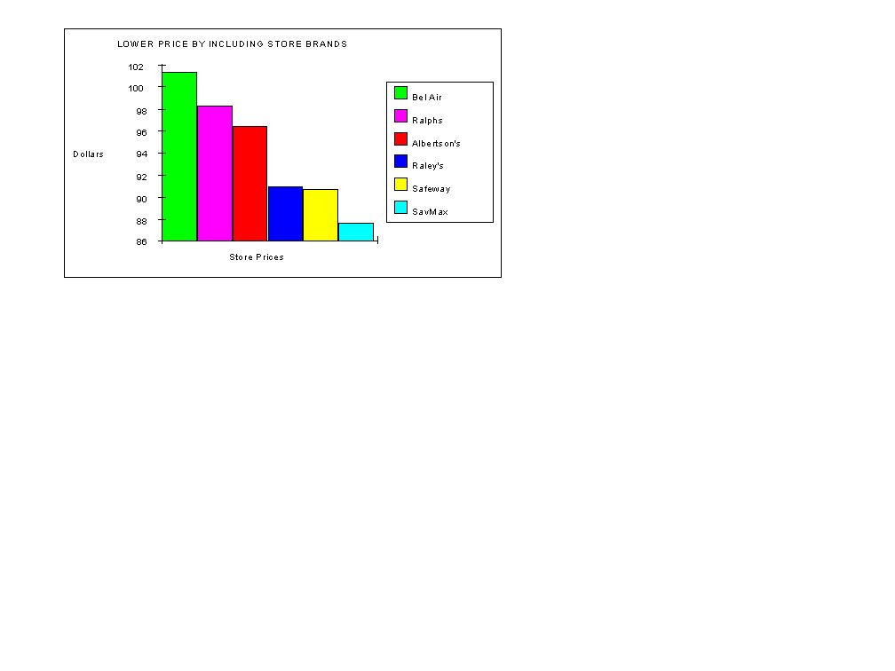To keep matters simple (usually but not always the best idea), I will stick to the shopping strategy which focuses on lowest prices (choosing store brands, along with all sale prices). In such a comparison, in Slice 1 the Shopping Cart at Bel Air totaled $101.40 to Raley's $90.97. The Final Slice found these two stores closer together with totals of $102.00 and $98.62, respectively. 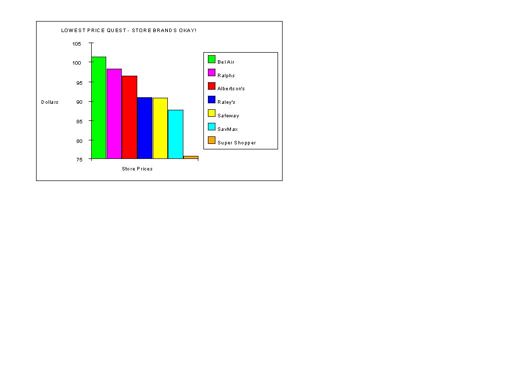Safeway was the Final Slice low price winner for folks who are willing to join their club and stock up (by buying two when the offer is "Buy One, Get One Free." The lowest prices on the Shopping Cart for Slice 1 were SavMax ($87.67) and Safeway ($90.75); and for the Final Slice, Safeway ($88.27) and SavMax ($90.57). The Super Shopper's quest for lowest prices for the Shopping Cart was consistently just under $76.00 in both slices. For Excel spreadsheets showing Shopping Cart lowest prices due to buying store brands and discounted items, click on:  Slice 1 or Final Slice.

               Click to see a map showing the supermarket locations. (This map is a reminder only; it's the same as the "final map" above.)

               Click on the supermarkets to see a photo:  Albertson's, Bel Air, Raley's, Ralphs, Safeway, and SavMax

                Different Strokes for Different Folks.  People are different. This study tries to compare prices for people who might make different choices in the market place. Some customers will stick with national or regional brand names, steering free of store brands for the most part. We show comparisons for these people -- when some of the items are on sale and what the price would have been if the full price had been charged.  Some customers focus only on prices; we show how they fare in their quest for "lowest price." If you look closely, you will even find the "super shopper," who goes from store to store, looking for the lowest of the low. Good luck on your sanity as you navigate the Slice 1 charts which follow!

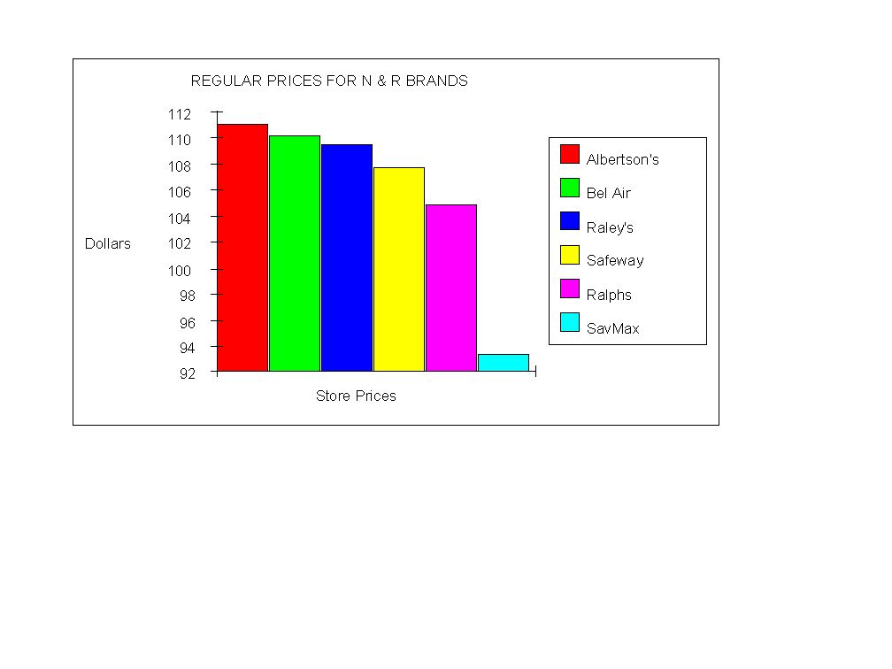
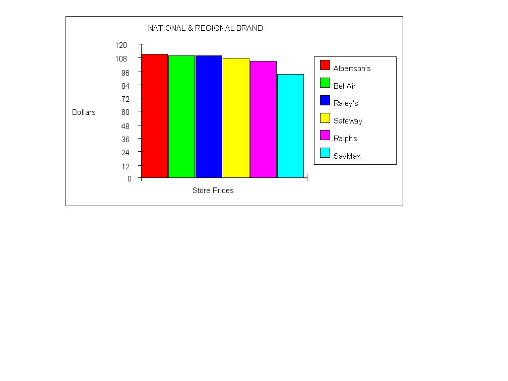
                Shopping cart total:  National and regional brand products at full price:  Compare!

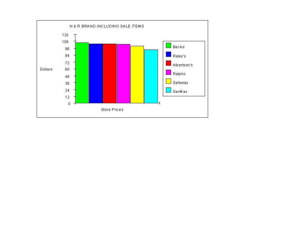
                Shopping cart total:  National and regional brand products with some sale items:  Compare!

                Shopping cart total:  Any brand to get the lowest price: Compare!

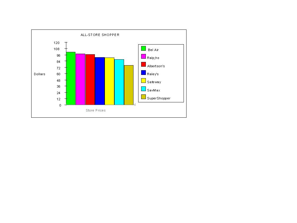
                Shopping cart total:  The determined super shopper saves a bundle of dollars (probably at extreme cost to everything else in her life!) by bouncing from store to store to find the lowest overall price.  Compare!

                A second look:  The above charts emphasize differences in total price.  Here is what Slice 1 price totals would look like when we chart from zero dollars:  N-R Brands, NRB with Sale Items, Low Price Leader.

Analysis

                The analysis of supermarket prices is difficult due to the many pricing strategies used by different stores. Price variables include store brands, simple sale prices (e.g., an item on sale for $1.79), complex sale prices (e.g., "buy one, get one free" or  "get $0.50 gift certificate with purchase of two cans of soup"), and "club" prices which exclude "nonmembers" from most sale items. The project tried to reflect prices as they would affect different types of customers: (1) those who would buy only well known national or regional brands, (2) those who would shop only a single store but always choose the "low price," and (3) those shoppers who are willing to shop multiple stores for the "super low price."
In this project, the "low price" shopper is  considered to be a customer who is willing to join the club, buy in quantity if necessary, or put up with anything in order to get the lower price. Coupons were not considered in the current study, because this factor is expected to apply across the board; no known instance of "double coupons" was encounered. No-label brands, overstocks, damaged containers, or close-dated perishable foods were not knowingly encountered during the project.

Conclusion

                No firm conclusions can be drawn at this time, except to note the simple, tentative comparisons above. For the most part, this project followed the advice expressed by DeMers (1997:428). Methodology furnished a framework.  Literature was reviewed. Field work was carried out properly and in a timely fashion. Computations were made. Analyses were a little flakey and can be improved upon. And the paper is written.

Disclaimer

                The conslusions above are tentative at best. The study is flawed in almost every direction. The comparisons made are only for the items selected for the study and only for the the time periods mentioned above. A different shopping list would result in differences in total prices. The data were checked for accuracy; still undetected errors are likely. In addition, prices make up only one of a number of factors which lead shoppers to one store instead of another. These include proximity (convenience of being nearby or on one's travel route), felt "cleanliness" or "orderliness," choice of products, customer-clerk-manager-store relations, and "ambiance" in general. A friend of mine once said, "Please don't ask me to read the ingredients or look at the prices."
 

References

Clarke, Keith C., 1997. Getting Started with Geographic Systems. Upper Saddle River, New Jersey: Prentice Hall, Inc.

DeMers, Michael N., 1997. Fundamentals of Geographic Information Systems. New York: John Wiley & Sons, Inc.

ESRI, 1997. Getting to Know ArcView GIS. Redlands, California: Environmental Systems Research Institute, Inc.

Hernandez, Michael J., 1997. Database Design for Mere Mortals.  Berkeley, California: Addison-Wesley Developers Press.

Hohl, Pat, ed., 1998.  GIS Data Conversion. Santa Fe, New Mexico: OnWord Press.

Robinson, Arthur H.,  Joel L. Morrison, Phillip C. Muehrcke, A. Jon Kimerling, and Stephen C. Guptill, 1995. Elements of Cartography, 6th edition. New York: John Wiley & Sons, Inc.